
Introduction
Most lotic waters provide a variety of habitats that create niches for heterogeneous vegetation. Medium-sized rivers in particular provide perfect conditions for highly diverse hydrophyte vegetation (Hussner & Lösch 2005). Species composition and abundance of freshwater macrophytes in lotic waters are determined by a few physical and chemical factors, such as current velocity (Janauer et al. 2010; Steffen et al. 2014), water depth (Steffen et al. 2014) and water chemistry (Riis et al. 2000; Coops et al. 2007; Maggioniet al. 2009) as well as grain size and nutrient content of the bottom sediments (Riis et al. 2000; Matsui 2014). Moreover, the water regime, described by duration, frequency as well as the rate of filling and drying, is an important factor determining the development of plant communities and patterns of vegetation zonation in aquatic ecosystems (Barrat-Segretain & Cellot 2007). Furthermore, the anthropogenic influence, land use in the riparian zone and bank structure are the most important parameters for the formation of macrophyte communities (Ot’ahel’ová et al. 2007). Ecosystems disturbed by human impact are more prone to invasions of alien species than undisturbed ecosystems, because plant communities in such conditions become more susceptible to invasion of non-native species (Hussner et al. 2010; Kolada & Kutyła 2016).
Elodea canadensis Michx. (Canadian waterweed) is an alien, invasive macrophyte species originating from North America (Hussner 2012). E. canadensis was first noted in Europe in 1836 in Great Britain (Moore and More 1866, reviewed in Simpson 1984) and recently, it is one of the most widespread alien aquatic plants, reported in 41 European countries (Hussner 2012). In some countries, this species rapidly spreads and displaces native species (Hussner et al. 2010; Mjelde et al. 2012), while in others, it does not demonstrate its invasive nature (Josefsson & Andersson 2001; Kuhar et al. 2010). Kolada & Kutyła (2016) also did not confirm the invasive nature of Canadian waterweed in Polish lakes and pointed to its non-aggressive integration with native vegetation.
E. canadensis is a cosmopolitan, submerged macrophyte rooted in sediment and playing an important role in the ecology of many littoral zones (Simpson 1986; Carbiener et al. 1990; Kähkönen & Manninen 1998; Janauer et al. 2010). It is capable of quick vegetative reproduction by stem fragments and overwintering buds (turions), which are easily dispersed by currents and animals (Barrat-Segretain 2001). It has a very high ecological tolerance and can be found in all kinds of water except salt water and waters extremely deficient in organic substances (Kłosowski & Kłosowski 2007). According to Szoszkiewicz et al. (2010b) and Haury et al. (2006), it can be found in waters with average nutrient content, ranging from mesotrophic to eutrophic ones. In rivers of northwest Germany, however, E. canadensis is also associated with soft water (Steffen et al. 2014). According to Kuhar et al. (2010), in Slovenia, E. canadensis prefers rivers flowing through agricultural landscapes, with a narrow, disturbed riparian zone and sediment consisting of gravel, sand, and silt with either coarse or fine organic matter particles. The species studied has been successfully employed in testing the accumulation of selected heavy metals (e.g. Ni, Cr) and enantiomers of organophosphorus pesticides, p’-DDT and o, p’-DDT, through its roots and the whole plant (Kähkönen & Manninenem 1998; Garrison et al. 2000; Jianping et al. 2000; Thiébaut et al. 2010; Hansen et al. 2011). According to Karen et al. (1998) and Garrison et al. (2000), it can be used for phytoremediation of polluted sites due to its ability to accumulate toxic chemicals and thus to remove them from the environment. Busuioc et al. (2012) also proved that E. canadensis is highly capable of accumulating Fe, Co, Zn, and Cu. According to Samecka-Cymerman & Kempers (2003), the positive correlations between the amount of Al, Cr, and Cu in bottom sediments and plant material confirm the usefulness of E. canadensis in monitoring the level of river pollution with these metals. Kolada & Kutyła (2016) examined E. canadensis in Polish lakes and demonstrated that the occurrence of this aquatic species in lake ecosystems is determined by altitude and water quality. These important results have prompted us to explore this problem in Polish rivers, the more that the Canadian waterweed is an invasive species and plays an important role in ecosystems as a bioaccumulator of trace metals and organic compounds (Kähkönen & Manninenem 1998; Garrison et al. 2000; Jianping et al. 2000; Thiébaut et al. 2010; Hansen et al. 2011). Although several studies on E. canadensis in rivers have been carried out (Szoszkiewicz et al. 2010a; Wiegleb et al. 2014; 2015; O’Hare et al. 2006), surveys on such a large scale in rivers have not yet been carried out in Poland. The presented results are based on the largest database of rivers in Poland, surveyed by a single team, using the same methods. The main objectives of this work were to investigate the range of habitat conditions (in terms of chemistry and hydromorphological parameters) at river sites colonized by E. canadensis and to analyze the accompanying species.
Materials and methods
Study area
The study was based on a countrywide survey conducted in Poland, with a dataset for 1135 river sites (Fig. 1). We analyzed 206 sites with Elodea canadensis, located in 173 water courses (the full list is presented in Appendix 1). The database was completed between 2003 and 2014. The basic parameters describing the studied rivers containing E. canadensis are presented in Table 1 (altitude, width and depth of a riverbed, bottom sediments, flow types, river valley land use, physical and chemical water parameters, and hydromorphological parameters) and in Table 2 (concentrations of macroelements and trace metals in water).
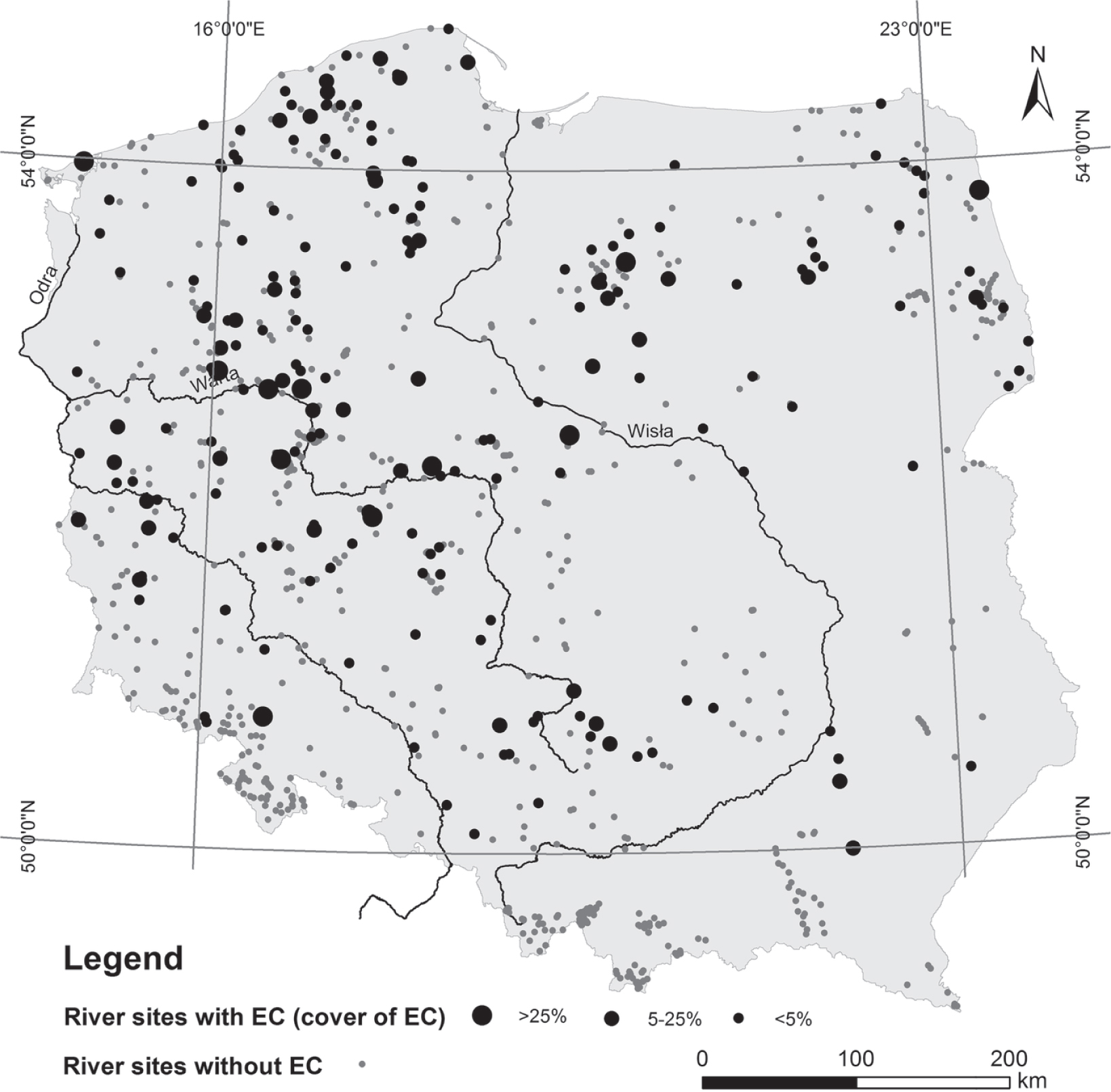
Figure 1
Distribution of the surveyed river sites (N = 206)
Table 1
Descriptive statistics of major habitat characteristics of the surveyed rivers (N = 206)
| Environmental variables | Units | Min. | Median | Max | Coefficient variation |
|---|---|---|---|---|---|
| Physical and chemical parameters of water | |||||
| pH | - | 6.90 | 7.76 | 9.30 | 0.04 |
| Alkalinity | mg CaCO3 l-1 | 37 | 165 | 490 | 0.36 |
| Conductivity | μS cm-1 | 192 | 449 | 2990 | 0.60 |
| Total phosphorus | mg P l-1 | 0.02 | 0.19 | 3.47 | 1.48 |
| Reactive phosphorus | mg PO43- l-1 | 0.02 | 0.35 | 8.58 | 1.80 |
| Nitrate nitrogen | mg N l-1 | 0.01 | 0.57 | 12.90 | 1.48 |
| Ammonium nitrogen | 0.00 | 0.16 | 12.96 | 2.78 | |
| Dimensions of a riverbed | |||||
| Average width | m | 1.5 | 5.5 | 45.0 | 0.97 |
| Average depth | 0.13 | 0.59 | 1.65 | 0.54 | |
| Hydromorphological metrics | |||||
| Altitude | m a.s.l. | 1 | 97 | 464 | 0.65 |
| HQA index | 0-100 | 15 | 39 | 79 | 0.34 |
| HMS index | 0-120 | 0 | 29 | 109 | 0.93 |
| RHQ index | 50-600 | 107 | 305 | 490 | 0.25 |
| RHM index | 0-240 | 0 | 34 | 174 | 0.98 |
| Shading of riverbed | % | 0 | 12 | 90 | 1.15 |
| Bottom sediments | |||||
| Granulometry index | 1-6 | 1.00 | 2.09 | 5.00 | 0.30 |
| Cobble | 0 | 0 | 53 | 2.69 | |
| Gravel/pebble | 0 | 10 | 93 | 1.21 | |
| Sand | % | 0 | 57 | 100 | 0.56 |
| Silt | 0 | 7 | 100 | 1.35 | |
| Peat | 0 | 0 | 93 | 5.85 | |
| Anthropogenic | 0 | 0 | 100 | 3.00 | |
| Flow types | |||||
| Flow type index | 1-6 | 1.00 | 1.51 | 4.13 | 0.42 |
| Chute | 0 | 0 | 19 | 1.82 | |
| Broken standing waves | 0 | 0 | 10 | 3.21 | |
| Unbroken standing waves | % | 0 | 0 | 58 | 2.21 |
| Rippled | 0 | 13 | 93 | 1.04 | |
| Smooth | 0 | 63 | 100 | 0.49 | |
| No perceptible flow | 0 | 3 | 100 | 1.79 | |
| Land use in a river valley | |||||
| Forest | 0 | 19 | 100 | 0.92 | |
| Wetland | % | 0 | 0 | 74 | 1.75 |
| Grassland | 0 | 30 | 100 | 0.80 | |
| Arable land | 0 | 0 | 81 | 1.56 | |
| Urban area | 0 | 0 | 100 | 1.63 | |
Table 2
Descriptive statistics of concentrations of elements in water of selected Elodea canadensis rivers (based on data from the State Environmental Monitoring)
| Elements | Units | Min. | Median | Max | Coefficient variation |
|---|---|---|---|---|---|
| Al (aluminum) | μg Al l-1 | 5 | 24 | 370 | 1.38 |
| As (arsenic) | μg As l-1 | 0.3 | 1.3 | 32.5 | 1.54 |
| B (boron) | μg B l-1 | 9 | 26 | 409 | 1.09 |
| Ba (bar) | μg Ba l-1 | 5 | 35 | 108 | 0.66 |
| Ca (calcium) | mg Ca l-1 | 19.4 | 79.6 | 191.1 | 0.37 |
| Cd (cadmium) | μg Cd l-1 | 0.01 | 0.10 | 7.70 | 2.64 |
| Cl (chlorine) | mg Cl- l-1 | 3.5 | 17.6 | 440.1 | 1.52 |
| Cr (chromium) | μg Cr l-1 | 0.02 | 0.63 | 42.50 | 2.23 |
| Cu (cooper) | μg Cu l-1 | 0.20 | 2.77 | 101.00 | 2.08 |
| F (fluorine) | mg F- l-1 | 0.02 | 0.18 | 1.75 | 1.18 |
| Fe (iron) | μg Fe l-1 | 1 | 133 | 1172 | 1.06 |
| Hg (mercury) | μg Hg l-1 | 0.01 | 0.10 | 3.28 | 1.87 |
| K (potassium) | mg K l-1 | 0.2 | 4.0 | 30.0 | 0.99 |
| Mg (magnesium) | mg Mg l-1 | 2.0 | 9.9 | 35.8 | 0.57 |
| Mn (manganese) | μg Mn l-1 | 2 | 110 | 492 | 0.85 |
| Na (sodium) | mg Na l-1 | 0.7 | 9.5 | 247.0 | 1.67 |
| Ni (nickel) | μg Ni l-1 | 0.25 | 2.50 | 34.73 | 1.35 |
| Pb (lead) | μg Pb l-1 | 0.20 | 2.50 | 33.00 | 1.48 |
| S (sulfur) | mg SO42- l-1 | 4.6 | 44.9 | 342.9 | 0.82 |
| Se (selenium) | μg Se l-1 | 0.3 | 2.9 | 25.0 | 1.05 |
| Zn (zinc) | μg Zn l-1 | 0.3 | 10.0 | 244.8 | 1.89 |
Macrophyte surveys
Macrophyte surveys were carried out during the intensive growth of most aquatic plants (from mid-June to mid-September). Field surveys were conducted using the Macrophyte Method for River Assessment (Szoszkiewicz et al. 2010b). This method is currently an official monitoring approach to rivers in Poland (Dziennik Ustaw 2016). The macrophyte assessment was based on the presence of algae, mosses, horsetails, liverworts, monocotyledonous and dicotyledonous plant species that are biological indicators of water quality. All submerged, free floating, semi-terrestrial and emergent plants were considered. The assessment also included macrophytes attached to or rooted in parts of the river bank substrate where they were likely submerged for most of the year. In wadeable survey sites, an aquascope was used to support the observations. The macrophyte survey was conducted over reaches of 100 m length. The survey includes a list of species and estimated ground cover of plants. The presence of each species was recorded with their percentage cover using the following nine-point scale: < 0.1%, 0.1-1%, 1-2.5%, 2.5-5%, 5-10%, 10-25%, 25-50%, 50-75% and > 75%. Based on the collected field data, the numerical index MIR (Macrophyte Index for Rivers) was computed (Szoszkiewicz et al. 2010b). It reflects river degradation, especially eutrophication and ranges from 10 (most degraded rivers) to 100 (highest quality). To assess the ecological status of the river, the calculated values of the MIR index were referenced to the current standards (Dziennik Ustaw 2016).
Hydrochemical parameters
During plant and hydromorphological surveys, three subsamples of water were randomly collected from each river site in the river midstream at a depth of 0.5-1 m. Water samples were not collected during rainy weather or periods with heavy runoff; if necessary, an additional visit was organized. Prior to analysis, all water samples were filtered using Sartorius cellulose filters with a nominal pore size of 0.45 μm, except for those used for the determination of total phosphorus. Water samples were cooled below 10°C and all parameters were analyzed in a laboratory within a 12h period. Electrical conductivity and pH were measured by digital potentiometers. Alkalinity was measured with sulfuric acid to the end point pH of 4.5 in the presence of methyl orange. Concentrations of phosphate (molybdenum blue method), total phosphorus (molybdenum blue method after microwave mineralization in MARS 5X), nitrate nitrogen (cadmium reduction method), and ammonium nitrogen (Nessler’s method) were determined using a spectrophotometer HACH DR/2800.
Information about concentrations of 21 elements in water was obtained from the State Environmental Monitoring. The research was carried out in laboratories accredited by the Polish Centre for Accreditation. Table 2 shows the average annual values as a mean of twelve measurements (Ca2+, Mg2+, Cl−, F−, and SO42−), or as a mean of four measurements (Al, As, B, Ba, Cd, Cr, Cu, Fe, Hg, K, Mn, Na, Ni, Pb, Se, and Zn).
Calcium and magnesium were determined by titration with EDTA (PN-ISO 6058:1999, PN-ISO 6059:1999) or by atomic absorption spectrometry (PN-EN ISO 7980:2002); sodium and potassium were measured by atomic absorption spectrometry (PN-ISO 9964-2:1994); chlorides were analyzed using the Mohr method, i.e. titration with silver nitrate in the presence of chromate as indicator (PN-ISO 9297:1994); sulfur was determined gravimetrically with barium chloride (PN-ISO 9280:2002); fluorides were measured using ion chromatography (PN-EN ISO 10304-1:2009). Trace elements were determined by atomic emission spectrometry with inductively coupled plasma (PN-EN ISO 11885:2009) and by atomic absorption spectrometry with a graphite tube (PN EN ISO 15586:2005) or with flame atomization (PN ISO 8288:2002). Mercury was determined by atomic fluorescence spectrometry with amalgamation enrichment (PN-EN ISO 17852:2009).
Measurement accuracy was determined by comparing the results of the determination of three separated portions of each sample, which were analyzed using the identical methods. Blank samples were digested in the same manner.
Hydromorphological surveys
Hydromorphological evaluation was conducted at each site according to the River Habitat Survey (RHS) method (Environment Agency 2003; Szoszkiewicz et al. 2012). The RHS data were collected from 500 m stretches of rivers. The RHS surveys were performed in ten profiles (spot checks) distributed at 50 m intervals. The macrophyte survey section was located inside each RHS site, always between the 6th and 8th spot check. Four numerical metrics based on the RHS protocol were produced: Habitat Quality Assessment– HQA, Habitat Modification Score – HMS (Raven et al. 1998; Szoszkiewicz et al. 2012), River Habitat Quality – RHQ, and River Habitat Modification – RHM (Tavzes & Urbanic 2009). The range of variability of the analyzed hydromorphological indices is given in Table 1. High values of HQA and RHQ indicate an extensive presence of a number of natural river features and high landscape diversity along the river. High HMS and RHM values indicate extensive anthropogenic alteration such as bank and channel re-sectioning and reinforcement or other river engineering constructions. The grain size composition and flow types were derived from the RHS database. Six flow types and six types of riverbed material were distinguished (Table 1). We also calculated the granulometry index and the flow type index (Jusik et al. 2015).
The granulometry index (GMindex) reflects the average grain size composition of the riverbed associated with the kinetic energy of the flow. It is based on the parameter “dominant channel substrate in spot checks” assessed using the RHS method (section E).
The flow type index (FTindex) reflects the average riverbed hydraulic characteristics associated with parameters such as slope, flow velocity and depth. It is based on the parameter “dominant flow type in spot checks” by the RHS method (section E).
Statistical analysis
Factor analysis (principal components analysis –PCA) with varimax normalized rotation was used to uncover the structure of environmental matrices and reveal environmental gradients. The ecological amplitude of E. canadensis was identified based on descriptive statistics of environmental variables (minimum, median, maximum and coefficient of variation). All calculations were performed with the Statistica 12.5 software (StatSoft Inc. 2014). Taxonomic diversity of macrophytes accompanying E. canadensis was analyzed using detrended correspondence analysis (DCA) from CANOCO for Windows version 4.55 (TerBraak & Smilauer 2002). Rare taxa found at up to three sampling sites were excluded from the analysis. DCA analysis of the biological data revealed that the first gradient length was 3.201 SD (standard deviation), indicating that the biological data exhibited unimodal responses to underlying environmental variables.
Results and discussion
Habitat description of rivers
Principal components analysis resulted in a simplified habitat description of the analyzed matrix. The first three factors were responsible for 43.5% of the sample variance. Table 3 presents three principal components and their corresponding eigenvalues after varimax normalized rotation; each of the three eigenvalues was responsible for more than 10% of the variance. The first principal component was strongly correlated with human impact, especially the degree of hydromorphological modification. It was negatively correlated with a percentage of urban areas, the RHM index, and the HMS index. The second principal component was strongly correlated with physicochemical water parameters reflecting the eutrophication. It was strongly positively correlated with total phosphorous, reactive phosphorous, and ammonia nitrogen. Finally, the third principal component was strongly correlated with high hydromorphological naturalness, forests as a land-use type and shading of a riverbed. The PCA results show that the analyzed database was characterized by a strong human impact gradient associated with hydromorphological modification of a riverbed and changes in land use and eutrophication. In the studied rivers, pH was the most stable environmental variable (CV = 0.04) and ammonium nitrogen – the most diverse one (CV = 2.78) (Table 2).
Table 3
Factor loadings of the first three principal components
| Environmental variables | Factorl | Factor 2 | Factor 3 |
|---|---|---|---|
| Physical and chemical parameters of water | |||
| pH | 0.198 | 0.089 | 0.199 |
| Alkalinity | 0.019 | 0.539 | -0.166 |
| Conductivity | -0.057 | 0.451 | -0.149 |
| Total phosphorus | -0.061 | 0.934* | -0.036 |
| Reactive phosphorus | -0.040 | 0.904* | 0.005 |
| Nitrate nitrogen | 0.041 | 0.094 | 0.013 |
| Ammonia nitrogen | -0.035 | 0.718* | -0.033 |
| Dimensions of a riverbed | |||
| Average width | 0.282 | -0.215 | 0.042 |
| Average depth | 0.213 | -0.281 | -0.248 |
| Hydromorphological metrics | |||
| Altitude | 0.106 | -0.149 | 0.060 |
| HQA index | 0.409 | -0.074 | 0.789* |
| HMS index | -0.759* | 0.001 | -0.361 |
| RHQ index | 0.614* | -0.174 | 0.150 |
| RHM index | -0.788* | -0.040 | -0.322 |
| Granulometry index | -0.423 | -0.195 | 0.432 |
| Flow type index | 0.127 | -0.192 | 0.595 |
| Shading of riverbed | 0.145 | 0.036 | 0.682* |
| Land use in a river valley at a distance of 50 m from the banks | |||
| Forests | 0.357 | -0.070 | 0.731* |
| Wetlands | 0.224 | -0.059 | 0.028 |
| Grassland | 0.482 | 0.050 | -0.617* |
| Arable land | -0.567 | 0.213 | -0.085 |
| Urban area | -0.819* | -0.127 | -0.021 |
| Eigenvalues (λ) | 3.546 | 3.048 | 2.967 |
| Percentage variance (%) | 16.1 | 13.9 | 13.5 |
Ecological amplitude of E. canadensis
E. canadensis occurs in lowland rivers throughout Poland (Fig. 1). It rarely occurs in upland rivers, and only up to an altitude of about 500 m a.s.l. (Table 1). The species was not found in mountain rivers. It prefers small and medium sandy lowland rivers (78% of the analyzed sites). Moreover, it occurs in gravelly lowland streams (14%), gravelly and sandy upland (7%) and stony siliceous upland watercourses (only three sites located in the Zadrna and Sopot rivers). The ecological status of the studied river sites, based on the MIR index, was as follows: 45% classified as good, 40% moderate, 8% very good and 7% poor. No Canadian waterweed sites were classified into bad ecological status.
Canadian waterweed has high light requirements and occurs mainly in unshaded sections of shallow rivers (often flowing through meadows) with an average depth of about 0.6 m (Table 1). It occurs in places with a dominant laminar flow (smooth) or slight turbulence (rippled). The median of the FTindex is 1.51. It avoids highly turbulent flow of high kinetic energy and marginal dead-water zones (Fig. 2). Waterweed occurs mostly in sandy bottom sections (median GMindex = 2.09), with some admixture of coarse mineral (gravel/pebble) and fine organic fraction (silt) (Fig. 3). It prefers moderately natural (HQA = 41 ± 14, RHQ = 307 ± 76) and moderately transformed (HMS = 32 ± 30, RHM = 40 ± 40) river sections, usually with a straightened planform, a uniform bank profile, re-sectioned and reinforced by fascines. It was not found in strongly transformed river sections (reinforced by concrete, sheet piling, cladding, cobblestones, and gabion) and those with reinforced banks and bottoms. E. canadensis was most often found in grasslands or forest river sections (Fig. 4), but moderately shady, on average 10-20% (Table 1).
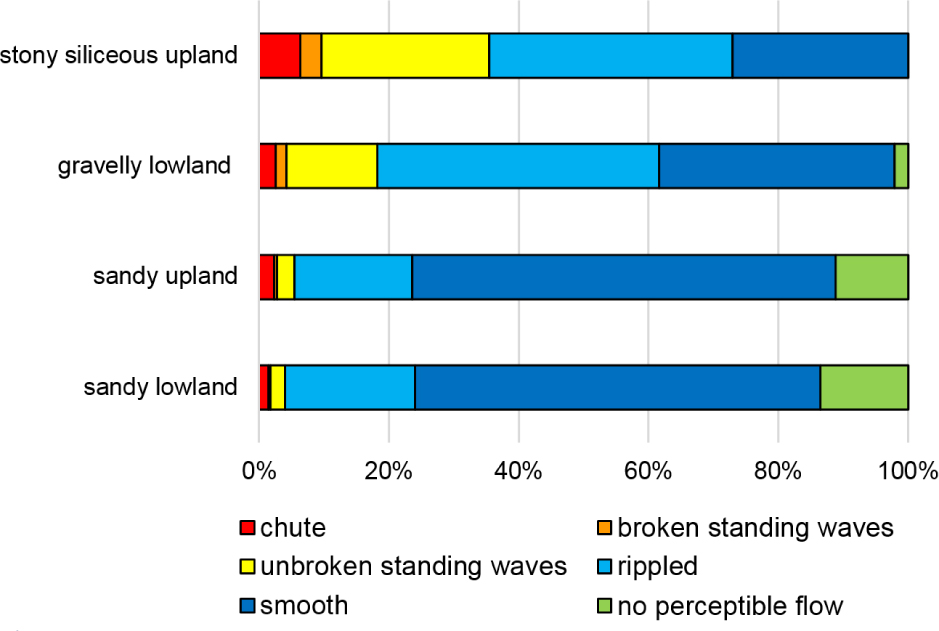
Figure 2
Percentage of each flow type (chute, broken standing waves, unbroken standing waves, rippled, smooth and no perceptible flow) in relation to all Elodea canadensis sites in four biocenotic types of rivers based on the RHS method (Environment Agency 2003; Szoszkiewicz et al.2012)
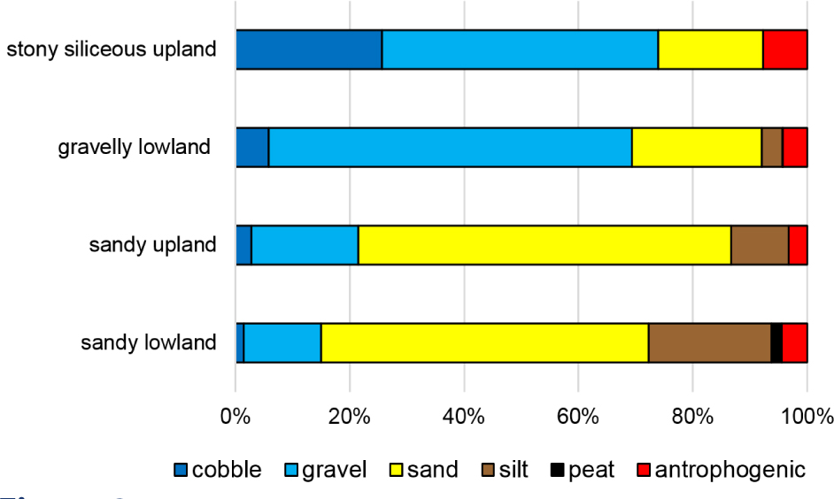
Figure 3
Percentage of each bottom sediment type (cobble, gravel, sand, silt, peat and anthropogenic) in relation to all Elodea canadensis sites in four biocenotic types of rivers based on the RHS method (Environment Agency 2003; Szoszkiewicz et al. 2012)
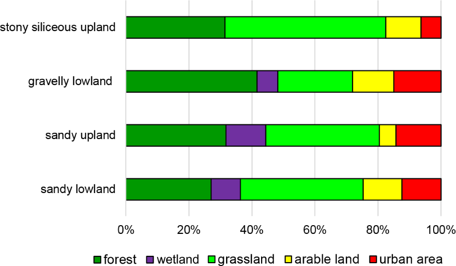
Figure 4
Percentage of each land-use type in river valleys (forest, wetlands, grassland, arable land, urban area) in relation to land use at all Elodea canadensis sites in four biocenotic types of rivers based on the RHS method (Environment Agency 2003; Szoszkiewicz et al. 2012)
In the present study, the pH of water from E. canadensis stands varied from 6.90 to 9.30 and was higher than the optimum range (pH 6-7) for the photosynthesis of E. nuttallii (Jones et al. 2000), which has very similar ecological and physiological requirements (Barrat-Segretain 2001). This is consistent with Santos et al. (2011), who stated that biomass of Canadian waterweed is positively correlated with pH. According to Santos et al. (2011), E. canadensis shows a higher growth rate and higher cover in areas with high conductivity, thus higher salinity. Also in the present study, Canadian waterweed prefers moderately mineralized water (545 ± 329 μS cm−1), rich in calcium and magnesium carbonates (174 ± 63 mg CaCO3 l−1, 84.1 ± 31.4 mg Ca2+ l−1 and 11.1 ± 6.4 mg Mg2+ l−1), with moderate concentrations of chlorides and sulfates (38.9 ± 59.1 mg Cl- l−1 and 62.3 ± 50.9 mg SO42− l−1). The average concentrations of Cl- and SO42− in the surveyed rivers were similar to that in the water of the Wielkopolska district (Poland) where E. canadensis stands were examined by Samecka-Cymerman & Kempers (2003). It also tolerates considerable salinity of the water (up to 247 mg Na l−1, 440 mg Cl− l−1 and 343 mg SO42− l−1).
In terms of nutrients, E. canadensis prefers water from mesotrophic to eutrophic (0.70 ± 1.25 mg PO43- l−1, 1.17 ± 1.73 mg NNO3− l−1, and 0.44 ± 1.21 mg NNH4+ l−1). This is in accordance with Thiébaut (2005), Kuhar et al. (2010) and Zehnsdorf et al. (2015) who reported that E. canadensis grows successfully under a wide range of environmental conditions, ranging from mesotrophic to eutrophic ones. Also Kolada & Kutyła (2016) showed that E. canadensis is most frequently accompanied by phytocoenoses of submerged macrophytes typical of mesotrophic and meso-eutrophic conditions. On the other hand, Meilinger et al. (2005); Dodkins et al. (2012) as well as Samecka-Cymerman & Kempers (2003) reported that Canadian waterweed belongs to nutrient tolerant taxa and is associated with high nutrient enrichment. Thriving in eutrophic water is probably enabled by its tolerance to low light intensity, even though it also tolerates high light without photoinhibition (Madsen et al. 1991).
In the studied rivers, concentrations of trace metals were generally at low levels (Table 2) and were in ranges characteristic of clean water bodies (Kabata-Pendias 2011), although the content of metals in water from some study sites was very high, e.g.: 3.28 μg Hg l−1 (the Meszna river, site Kąty, 2006), 7.70 μg Cd l−1, 32.5 μg As l−1, 33.0 μg Pb l−1, and 101 μg Cu l−1 (the Kania river, site Gostyn, 2006), 245 μg Zn l−1, 409 μg B l−1, and 492 μg Mn l−1 (the Przemsza river, site Będzin, 2006). These metal concentrations were significantly higher than those determined in water of waterweed stands in Poland (Samecka-Cymerman & Kempers 2003) and in north-eastern France (Thiébaut et al. 2010).
Macrophyte species accompanying E. canadensis
The Detrended Correspondence Analysis (DCA) ordination of the macrophyte species is presented in Fig. 5 The first axis (λ1 = 0.303) can be identified with the kinetic energy of water (current velocity), which directly affects the degree of riverbed material fragmentation and the observed types of flow. Aquatic bryophytes and some filamentous algae (e.g. Hildenbrandia rivularis) as well as vascular macrophytes associated with the community of Ranunculion fluitantis (genera Batrachium and Callitriche) prefer more turbulent and fast flows, while floating-leaved macrophytes and pleustophytes – no flow (Fig. 5). The second axis (λ2 = 0.248) was correlated with the concentration gradient of nutrients in the water of the surveyed rivers.
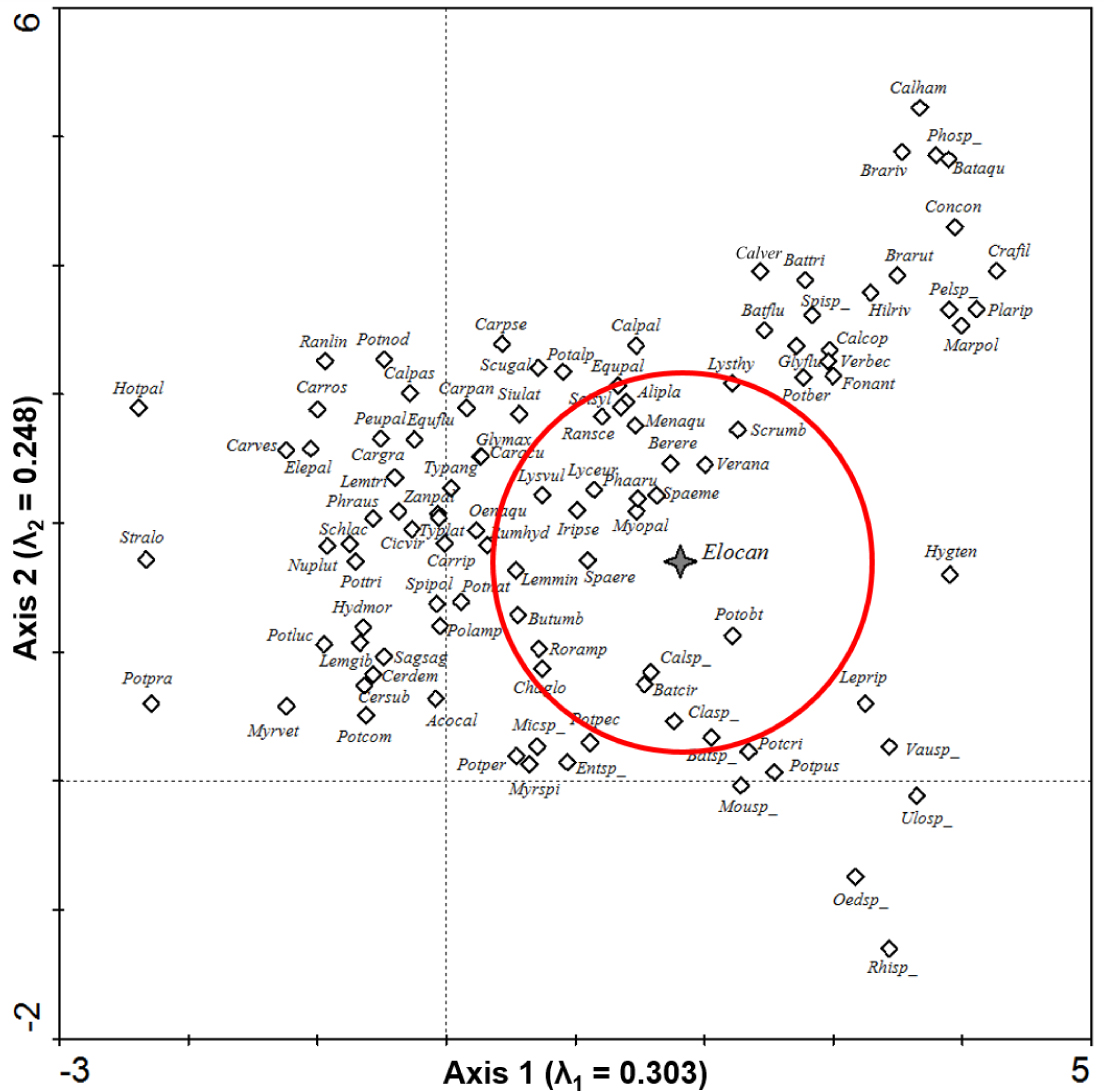
Figure 5
DCA ordination diagrams of macrophyte species. The circle indicates the most common species occurring with Elodea canadensis
For comparison, the CCA ordination diagrams of plant communities accompanying Elodea canadensis in Polish lakes examined during the State Environmental Monitoring (area > 50 ha) and presented in Kolada & Kutyła (2013), Fig. 4b
Abbreviations:
Acocal – Acorus calamus, Alipla – Alisma plantago-aquatica, Bataqu – Batrachium aquatile, Batcir – Batrachium circinatum, Batflu – Batrachium fluitans, Battri – Batrachium trichophyllum, Batsp_ – Batrachospermum sp., Berere – Berula erecta, Brariv – Brachythecium rivulare, Butumb – Butomusum bellatus, Calcop – Callitriche cophocarpa, Calham – Callitriche hamulata, Calpal – Caltha palustris, Calpas – Calla palustris, Calver – Callitriche verna, Calsp_ – Callitriche sp., Caracu – Carex acutiformis, Cargra – Carex gracilis, Carpan – Carexpaniculata, Carpse – Carex, Carrip – Carex riparia, Carros – Carex rostrata, Carves – Carex vesicaria, Cerdem – Ceratophyllum demersum, Cersub – Ceratophyllum submersum, Chaglo – Chara globularis, Cicvir – Cicuta virosa, Clasp_ – Cladophora sp., Concon – Conocephalum conicum, Crafil – Cratoneuron filicinum, Elepal – Eleocharis palustris, Elocan – Elodea canadensis, Entsp_ – Enteromorpha sp., Equflu – Equisetum fluviatile, Equpal – Equisetum palustre, Fonant – Fontinalis antipyretica, Glyflu – Glyceria fluitans, Glymax – Glyceria maxima, Hilriv – Hildenbrandia rivularis, Hotpal – Hottonia palustris, Hydmor – Hydrocharis morsus-ranae, Hygten – Hygroamblystegium tenax, Iripse – Iris pseudacorus, Lemgib – Lemna gibba, Lemmin – Lemna minor, Lemtri – Lemna trisulca, Leprip – Leptodictyum riparium, Lyceur – Lycopus europaeus, Lysthy – Lysimachia thyrsiflora, Lysvul – Lysimachia vulgaris, Marpol – Marchantia polymorpha, Menaqu – Mentha aquatica, Micsp_ – Microspora sp., Mousp_ – Mougeotia sp., Myopal – Myosotis palustris, Myrspi – Myriophyllum spicatum, Myrvet – Myriophyllum verticillatum, Nuplut – Nuphar lutea, Oedsp_ – Oedogonium sp., Oenaqu – Oenanthe aquatica, Pelsp_ – Pellia sp., Peupal – Peucedanum palustre, Phaaru – Phalaris arundinacea, Phosp_ – Phormidium sp., Phraus – Phragmites australis, Plarip – Platyhypnidium riparioides, Polamp – Polygonum amphibium, Potalp – Potamogeton alpinus, Potber – Potamogeton berchtoldii, Potcom – Potamogeton compressus, Potcri – Potamogeton crispus, Potluc – Potamogeton lucens, Potnat – Potamogeton natans, Potnod – Potamogeton nodosus, Potobt – Potamogeton obtusifolius, Potpec – Potamogeton pectinatus, Potper – Potamogeton perfoliatus, Potpra – Potamogeton praelongus, Potpus – Potamogeton pusillus, Pottri – Potamogeton trichoides, Ranlin – Ranunculus lingua, Ransce – Ranunculus sceleratus, Rhisp_ – Rhizoclonium sp., Roramp – Rorippa amphibia, Rumhyd – Rumexhydrolapathum, Sagsag – Sagittaria sagittifolia, Schlac – Schoenoplectus lacustris, Scisyl – Scirpus sylvaticus, Scrumb – Scrophularia umbrosa, Scugal – Scutellaria galericulata, Siulat – Sium latifolium, Spaeme – Sparganium emersum, Spaere – Sparganium erectum, Spipol – Spirodela polyrhiza, Spisp_ – Spirogyra sp., Stralo – Stratiotes aloides, Typang – Typha angustifolia, Typlat – Typha latifolia, Ulosp_ – Ulothrix sp., Vausp_ – Vaucheria sp., Verana – Veronica anagallis-aquatica, Verbec – Veronica beccabunga, Zanpal – Zannichellia palustris
E. canadensis occurs most often with vascular macrophytes associated with slow-flowing rivers with sandy bottom material, indicating mesotrophic and eutrophic water (Fig. 5). In the studied material, the Canadian waterweed occurred accompanied by 105 taxa of macrophytes, including 13 macroscopic algae, 11 bryophytes and 81 vascular plants. The most dominant emergent species were (Fig. 5): Alisma plantago-aquatica, Berula erecta, Butomus umbellatus, Iris pseudacorus, Lycopus europaeus, Lysimachia vulgaris, Mentha aquatica, Myosotis palustris, Phalaris arundinaceae, Ranunculus sceleratus, Rorippa amphibia, Scrophularia umbrosa, Sparganium emersum, S. erectum, and Veronica anagallis-aquatica. Among submerged plant species, Batrachium circinatum and Potamogeton obtusifolius were most common, while among pleustophytes, Lemna minor dominated. The filamentous algae Cladophora sp. also occurred, a tolerant taxon which is an indicator of eutrophication (Haury et al. 2006; Szoszkiewicz et al. 2010b).
Comparison of E. canadensis in rivers and lakes
The average contribution of E. canadensis in the lake phytolittoral varied between 2.3 and 5.5% (Kolada & Kutyła 2016) and was similar to its average contribution in the studied rivers (5.9%), although the species was more common in lakes (40% of the studied lakes) studied by Kolada & Kutyła (2016) than in rivers (26% of the studied river sites). The reason may be greater heterogeneity of habitat conditions in lotic ecosystems.
In terms of abiotic factors, E. canadensis prefers deeper and larger lakes, with a long water retention time, lower trophic status of waters and better ecological status (Kolada & Kutyła 2016). Other studies indicate that Canadian waterweed is common in water depths between 4 and 8 m (Nichols & Shaw 1986). However, Kłosowski et al. (2011) reported that E. canadensis phytocoenoses are associated with the shallowest parts of lakes. In the present study, it occurs more often in small and shallow streams (average depth of 0.6 m and width of 5.5 m). In terms of trophic and ecological status, the results obtained for the studied rivers and Portuguese rivers (Dodkins et al. 2012) were similar to those obtained for lakes – mesotrophic to eutrophic conditions and at least good ecological status (53% of all sites) (Kolada & Kutyła 2016). It should be added, however, that the conductivity and concentration of nutrients in water were higher in rivers than in lakes – the conductivity was on average 449 μS cm−1 in the studied rivers and 303 μS cm−1 in lakes (Kolada & Kutyła 2016), whereas the content of phosphorus was 0.19 mg P l−1 in rivers and 0.043 mg P l−1 (Kolada & Kutyła 2016) in lakes, respectively. Also alkalinity was slightly higher in rivers, on average 165 mg CaCO3 l−1, while in lakes it was 130 mg CaCO3 l−1 (Kolada & Kutyła 2016). On the other hand, average pH was higher in lakes – 8.3 (Kolada & Kutyła 2016) and 7.76 in rivers.
In the analyzed Polish lakes, 78 hydrophyte communities were identified. Elodea canadensis forms a compact plant community in the vicinity of other submerged phytocoenoses (elodeids and charids). The most common are plant communities such as: Charetum fragilis, Charetum rudis, Myriophyllum alterniflorum, Potametum alpinii, P.compressi, P.lucentis, P. obtusifolii, P. pusilli, Ranunculetum circinati (Kolada & Kutyła 2016). Macrophytes in rivers were assessed based on the Macrophyte Method for River Assessment, i.e. based on species rather than plant communities, so direct comparison with lakes is not possible. In addition, charids are a very important group in lakes (represented by e.g. Charetum fragilis and Charetum rudis), especially those with at least good ecological status, preferred by Elodea canadensis, while they are very rare in rivers. Only Chara globularis (syn. Chara fragilis) from this group was found in the studied rivers, at 4 sites. In total, 105 taxa of macrophytes were identified in rivers, including 81 vascular plants. Most of the studied rivers were dominated by relatively shallow sections (0.13-1.65 m, mean 0.59 m), therefore, the Canadian waterweed was accompanied by numerous emergent species – rushes, in addition to the submerged macrophytes (e.g. Batrachium circinatum, Potamogeton obtusifolius). The most important of them, occurring in at least 50% of the Elodea canadensis sites, were: Berula erecta, Mentha aquatica, Myosotis palustris, Sparganium emersum and Veronica anagallis-aquatica.
Conclusions
In summary, Elodea canadensis was commonly found in lowland rivers throughout Poland, but rarely in upland streams. The species has high light requirements and occurs mainly in unshaded sections of shallow rivers. It occurs in places with a dominant laminar flow (smooth) or slight turbulence (rippled), most often in sandy bottom sections of rivers, with some admixture of coarse mineral (gravel/pebble) and fine organic fraction. Canadian waterweed prefers sections of rivers that are moderately hydromorphologically transformed, usually with a uniform bank profile, re-sectioned and reinforced by fascines. It prefers moderately mineralized water, rich in calcium and magnesium carbonates, with moderate concentrations of chlorides and sulfates and mesotrophic to eutrophic conditions. Therefore, light and nutrient concentrations in water can be very important factors regulating the abundance and range of Canadian waterweed populations in Polish rivers. Elodea canadensis occurs mostly with vascular macrophytes associated with slow-flowing rivers, with sandy bottom material, indicating mesotrophic and eutrophic water.
Acknowledgements
This research was supported by the National Science Center of Poland, grant no. 2013/09/N/NZ8/03253 and by the University of Wroclaw (4740/PB/KEBOŚ/14 418) as well as by the Ministry of Science and Higher Education, grant no. 2 P04 G13629. The authors thank the following persons (in alphabetical order) for their help in field research: Dr. Daniel Gebler, MSc Artur Golis, Dr. Jerzy M. Kupiec, Dr. hab. Agnieszka E. Ławniczak (Professor at Poznań University of Life Sciences), MSc Dominik Mendyk, MSc Marcin Przesmycki, Dr. hab. Ryszard Staniszewski, MSc Marta Szwabińska; Dr. Tomasz Zgoła. We also thank the MSc students of Poznan University of Life Sciences.
Appendices
Appendix 1.
List of the surveyed river sites (N = 206) with Elodea canadensis. Geographical names are based on the National Register of Geographical Names and topographic maps on a scale of 1:10 000.
| No. | Name of the river | The nearest place | Province | Year of survey | Geographical coordinates | No. of a grid ATPOL square | Cover of E. canadensis* | |
|---|---|---|---|---|---|---|---|---|
| 1. | Baczyna | Lubin, ul. Sikorskiego | dolnośląskie | 2013 | 51°23′38.6″N | 16°12′14.1″E | BE13 | 2 |
| 2. | Biała (Biela) | Struga | lubuskie | 2008 | 52°06′34.8″N | 15°07′42.0″E | AD36 | 3 |
| 3. | Białka | Koniecpol | śląskie | 2011 | 50°45′43.2″N | 19°40′33.2″E | DE87 | 5 |
| 4. | BiałkaLelowska | Lelów | śląskie | 2010 | 50°41′09.2″N | 19°37′17.7″E | DE97 | 4 |
| 5. | Blizna | Szczebra | podlaskie | 2004 | 53°54′27.0″N | 22°58′49.3″E | FB29 | 2 |
| 6. | Błędzianka | PuszczaRomnicka | warmińsko-mazurskie | 2011 | 54°20′25.9″N | 22°35′03.7″E | FA86 | 3 |
| 7. | Bóbr | Żelisław | lubuskie | 2005 | 51°34′18.0″N | 15°24′43.0″E | AD98 | 1 |
| 8. | Brda | Piła - Młyn | kujawsko-pomorskie | 2005 | 53°30′49.2″N | 17°53′06.4″E | CB85 | 1 |
| 9. | Brda | Zapora (Mylof) | pomorskie | 2006 | 53°46′22.1″N | 17°43′07.6″E | CB54 | 3 |
| 10. | Bukówka (Kamionka) | Kuźniczka | wielkopolskie | 2005 | 52°56′46.1″N | 16°12′38.3″E | BC44 | 2 |
| 11. | Bytowa | Bytów | pomorskie | 2013 | 54°10′02.2″N | 17°29′04.0″E | CB03 | 4 |
| 12. | Chotla | ZaspyMałe | zachodniopomorskie | 2006 | 54°01′44.2″N | 16°09′30.5″E | BB14 | 1 |
| 13. | Ciemna | Tursko | wielkopolskie | 2009 | 51°52′19.4″N | 17°56′49.0″E | CD65 | 1 |
| 14. | Cieszynka | Bukowo | zachodniopomorskie | 2008 | 53°05′45.1″N | 16°11′55.6″E | BC24 | 5 |
| 15. | Cieszynka | Człopa, ul. Młyńska | zachodniopomorskie | 2008 | 53°05′23.1″N | 16°07′19.2″E | BC23 | 1 |
| 16. | Czapliniecka Struga | Czaplinek | zachodniopomorskie | 2013 | 53°33′43.3″N | 16°13′48.9″E | BB74 | 4 |
| 17. | Czarna | Okonek | wielkopolskie | 2011 | 53°32′08.3″N | 16°51′13.1″E | BB78 | 3 |
| 18. | Czarna Przemsza | Sosnowiec, ul. Będzińska | śląskie | 2006 | 50°17′51.8″N | 19°08′15.6″E | DF33 | 1 |
| 19. | Czarna Struga | Nowa Sól, os. Konstytucji 3 maja | lubuskie | 2013 | 51°48′20.3″N | 15°41 '32.1 "E | BD60 | 1 |
| 20. | Czarna Woda | Ostrowo | pomorskie | 2006 | 54°49′49.6″N | 18°14′22.8″E | CA38 | 3 |
| 21. | Czarna Woda | Sępolno | wielkopolskie | 2008 | 52°22′35.8″N | 16°00′40.7″E | BD02 | 2 |
| 22. | Czarnka | Opole, ul. Adama | opolskie | 2011 | 50°37′04.9″N | 17°59′37.0″E | CF05 | 4 |
| 23. | Czerska Struga | Czersk | pomorskie | 2013 | 53°47′33.0″N | 17°58′42.0″E | CB46 | 3 |
| 24. | Czerska Struga | Końskie Błota | pomorskie | 2006 | 53°43′04.0″N | 17°53′35.9″E | CB55 | 4 |
| 25. | Czerwona | Łasin Koszaliński | zachodniopomorskie | 2006 | 54°13′37.5″N | 15°48′06.6″E | BA92 | 1 |
| 26. | Dar (Sienica) | Dębno | zachodniopomorskie | 2008 | 52°44′44.1″N | 14°41 '28.1 "E | AC53 | 2 |
| 27. | Dobrzyca | Czapla | zachodniopomorskie | 2004 | 53°16′58.2″N | 16°34′07.2″E | BC06 | 5 |
| 28. | Dojca | Obra | wielkopolskie | 2008 | 52°04′29.3″N | 16°04′34.1″E | BD32 | 3 |
| 29. | dopływ Grabowej | Wielin (rez. Wieleń) | zachodniopomorskie | 2005 | 54°09′31.5″N | 16°42′27.7″E | BB08 | 4 |
| 30. | dopływ Krąpielicy (Młynówki) | Stargard Szczeciński, Park Panorama | zachodniopomorskie | 2013 | 53°20′30.9″N | 15°03′11.7″E | AB96 | 4 |
| 31. | Drawa | Sitnica | zachodniopomorskie | 2009 | 53°06′52.6″N | 15°53′24.2″E | BC22 | 6 |
| 32. | Dzierżęcinka | Koszalin, ul. Batalionów Chłopskich | zachodniopomorskie | 2007 | 54°12′21.8″N | 16°10′10.4″E | BB04 | 3 |
| 33. | Flinta | Jaracz | wielkopolskie | 2008 | 52°42′26.3″N | 16°51′41.5″E | BC68 | 8 |
| 34. | Flinta | Ryczywół | wielkopolskie | 2009 | 52°48′34.1″N | 16°50′45.0″E | BC58 | 2 |
| 35. | Flinta | Skrzetusz | wielkopolskie | 2005 | 52°50′43.4″N | 16°48′05.3″E | BC58 | 2 |
| 36. | Gizela (Gryżlina) | Zajączki | warmińsko-mazurskie | 2005 | 53°33′26.5″N | 19°52′57.9″E | DB78 | 2 |
| 37. | Główna | Mechowo | wielkopolskie | 2007 | 52°26′47.9″N | 17°02′55.9″E | BC99 | 2 |
| 38. | Główna | Poznań, ul. Hlonda | wielkopolskie | 2007 | 52°25′32.4″N | 16°57′56.3″E | BD09 | 1 |
| 39. | Gniły Potok | Mościsko | dolnośląskie | 2011 | 50°46′52.8″N | 16°35′35.4″E | BE86 | 9 |
| 40. | Grabiczek | Grabin | warmińsko-mazurskie | 2004 | 53°37′40.3″N | 20°02′25.3″E | DB69 | 2 |
| 41. | Grabowa | Sulechówko | zachodniopomorskie | 2011 | 54°16′25.8″N | 16°33′54.9″E | BA97 | 6 |
| 42. | Graniczna | Żarkowo | pomorskie | 2011 | 54°22′31.7″N | 17°19′40.0″E | CA82 | 3 |
| 43. | Gryżynka (Gryżyński Potok) | Grabin | lubuskie | 2003 | 52°07′23.7″N | 15°16′45.9″E | AD27 | 2 |
| 44. | Gwda | Piła - Kalina | wielkopolskie | 2009 | 53°06′18.7″N | 16°47′02.9″E | BC28 | 1 |
| 45. | Ilanka | Maczków | lubuskie | 2004 | 52°16′17.7″N | 14°45′32.3″E | AD14 | 1 |
| 46. | Iławka | Młody Bór | warmińsko-mazurskie | 2007 | 53°32′14.4″N | 19°40′15.4″E | DB77 | 4 |
| 47. | Jerzgnia | Ciszewo | podlaskie | 2007 | 53°37′28.2″N | 22°42′11.7″E | FB67 | 1 |
| 48. | Kanal Nowa Ulga | Warszawa, os. Iskra | mazowieckie | 2013 | 52°13′13.8″N | 21°06′03.4″E | ED27 | 4 |
| 49. | Kanał Augustowski | Białobrzegi | podlaskie | 2012 | 53°48′18.3″N | 22°57′57.8″E | FB49 | 3 |
| 50. | Kanał Grójecki | Wola Podłężna | wielkopolskie | 2012 | 52°14′27.2″N | 18°20′42.0″E | CD28 | 2 |
| 51. | Kanał Lodowy | Gidle | łódzkie | 2007 | 50°57′19.1″N | 19°28′13.6″E | DE66 | 5 |
| 52. | Kanał Łeby | Cecenowo | pomorskie | 2006 | 54°39′03.3″N | 17°33′29.8″E | CA53 | 6 |
| 53. | Kanał Łęg - Klewiec | Krawce | podkarpackie | 2014 | 50°31′15.2″N | 21°53′47.3″E | FF13 | 4 |
| 54. | Kanał Młyński | Słupsk | pomorskie | 2011 | 54°27′44.7″N | 17°02′17.3″E | CA70 | 2 |
| 55. | Kanał Słupi | Słupsk | pomorskie | 2011 | 54°26′55.9″N | 17°01′58.4″E | CA70 | 6 |
| 56. | Kanał Turośl | pow. Turośli | podlaskie | 2011 | 53°23′34.4″N | 21°44′05.3″E | FB91 | 1 |
| 57. | Kanał Warty | Częstochowa | śląskie | 2011 | 50°48′19.0″N | 19°08′03.8″E | DE83 | 1 |
| 58. | Kanał Zuzanka | Włocławek, ul. Graniczna | pomorskie | 2013 | 52°38′52.8″N | 19°08′30.5″E | DC73 | 3 |
| 59. | Kania | Gostyń, ul. Fabryczna | wielkopolskie | 2013 | 51°52′53.2″N | 17°01′14.3″E | BD69 | 5 |
| 60. | Kania | pon. Gostynia | wielkopolskie | 2008 | 51°54′36.4″N | 17°00′54.2″E | BD59 | 3 |
| 61. | Kicz | Tuchola | kujawsko-pomorskie | 2013 | 53°35′13.9″N | 17°51′21.8″E | CB75 | 2 |
| 62. | Kirsna | Swajnie | warmińsko-mazurskie | 2006 | 54°01′28.5″N | 20°30′17.8″E | EB22 | 3 |
| 63. | Kisewa (Kisewska Struga) | Nowa Wieś Lęborska | pomorskie | 2013 | 54°33′30.8″N | 17°43′45.1″E | CA64 | 4 |
| 64. | Kłoniecznica | Kłonecznica | pomorskie | 2011 | 53°58′48.1″N | 17°30′33.6″E | CB23 | 5 |
| 65. | Kłoniecznica | Mielno | pomorskie | 2009 | 53°56′34.9″N | 17°29′59.9″E | CB33 | 4 |
| 66. | Konopka | Częstochowa - Sabinów | śląskie | 2011 | 50°46′18.3″N | 19°05′43.0″E | DE83 | 3 |
| 67. | Kończak | Podlesie | wielkopolskie | 2004 | 52°45′02.4″N | 16°40′29.6″E | BC67 | 5 |
| 68. | Korytnica | Jaźwiny | zachodniopomorskie | 2004 | 53°10′00.2″N | 15°54′58.6″E | BC12 | 2 |
| 69. | Krztynia | Tęgobórz | śląskie | 2011 | 50°38′33.0″N | 19°47′57.4″E | DF08 | 5 |
| 70. | Krzycki Rów | Krzekotów | kujawsko-pomorskie | 2004 | 52°46′46.8″N | 17°59′12.2″E | CC66 | 5 |
| 71. | Kulawa | Laska | pomorskie | 2009 | 53°56′08.9″N | 17°32′01.9″E | CB33 | 6 |
| 72. | Kulawa | Wawrzonowo | pomorskie | 2011 | 53°57′08.8″N | 17°31′59.3″E | CB33 | 4 |
| 73. | Kwacza | Kwakowo (odc. nie renat.) | pomorskie | 2012 | 54°22′06.5″N | 17°01′10.0″E | CA80 | 4 |
| 74. | Kwacza | Kwakowo (odc. renat.) | pomorskie | 2012 | 54°22′32.6″N | 17°01′47.2″E | CA80 | 3 |
| 75. | Kwisa | Luboszów | dolnośląskie | 2006 | 51°25′53.9″N | 15°23′56.9″E | AE07 | 3 |
| 76. | Kwisa | T rzebów | lubuskie | 2007 | 51°33′02.7″N | 15°23′38.9″E | AD98 | 5 |
| 77. | Lega | Olecko, ul. Partyzantów | warmińsko-mazurskie | 2004 | 54°02′21.1″N | 22°30′31.2″E | FB15 | 1 |
| 78. | Leśna Prawa | Topiło (rez. Olszynka Mysliszcze) | podlaskie | 2004 | 52°38′50.8″N | 23°40′24.4″E | GC64 | 4 |
| 79. | Lewińska Struga | Kołczewo | zachodniopomorskie | 2014 | 53°58′44.8″N | 14°37′56.6″E | AB24 | 7 |
| 80. | Liswarta | Tanina | śląskie | 2007 | 50°45′13.7″N | 18°46′56.7″E | DE81 | 6 |
| 81. | Liśnica | Białogard, ul. Nadbrzeżna | zachodniopomorskie | 2013 | 54°00′14.3″N | 15°59′02.8″E | BB23 | 2 |
| 82. | Liwiec | Nadkole | mazowieckie | 2005 | 52°35′25.1″N | 21°35′09.1″E | FC80 | 3 |
| 83. | Lubsza (Lubica) | Stargard Gubinski | lubuskie | 2006 | 51°53′01.6″N | 14°47′13.1″E | AD54 | 6 |
| 84. | Lutynia | Wilkowyja | wielkopolskie | 2006 | 51°59′41.1″N | 17°32′17.5″E | CD42 | 6 |
| 85. | Lutynia | Wola Książęca | wielkopolskie | 2006 | 51°57′57.1″N | 17°34′12.2″E | CD53 | 7 |
| 86. | Łabianka | Łabno | podlaskie | 2007 | 53°24′18.5″N | 21°56′28.9″E | FB82 | 1 |
| 87. | Łącza (Złoty Potok) | Czerwieńsk | lubuskie | 2005 | 52°00′46.7″N | 15°25′32.6″E | AD48 | 6 |
| 88. | Łupawa | Smołdzino, ul. Mostowa | pomorskie | 2011 | 54°39′43.2″N | 17°12′48.6″E | CA51 | 2 |
| 89. | Łutownia | Stara Bialowieża | podlaskie | 2004 | 52°44′01.8″N | 23°47′07.9″E | GC55 | 3 |
| 90. | Mała Panew | Brusiek | śląskie | 2009 | 50°34′49.3″N | 18°49′15.8″E | DF01 | 1 |
| 91. | Mała Wełna | Kiszkowo | wielkopolskie | 2004 | 52°35′23.5″N | 17°16′05.6″E | CC81 | 5 |
| 92. | Mała Wkra (Wikierka) | Stare Miasto | warmińsko-mazurskie | 2009 | 53°27′52.4″N | 20°00′22.7″E | DB89 | 7 |
| 93. | Meszna | Dziedzice-Kąty | wielkopolskie | 2007 | 52°14′34.8″N | 17°50′38.1″E | CD25 | 2 |
| 94. | Miała | Kamiennik | wielkopolskie | 2006 | 52°48′31.7″N | 15°59′03.3″E | BC52 | 3 |
| 95. | Miała | Piłka | wielkopolskie | 2004 | 52°47′44.1″N | 16°03′07.9″E | BC53 | 7 |
| 96. | Mierzawa | Słaboszowice | świętokrzyskie | 2007 | 50°35′13.6″N | 20°11′13.4″E | EF01 | 2 |
| 97. | Mierzawa | Tarnawa | świętokrzyskie | 2014 | 50°33′55.8″N | 20°02′56.8″E | EF00 | 2 |
| 98. | Mławka | Szreńsk | mazowieckie | 2004 | 53°00′31.6″N | 20°07′40.9″E | EC30 | 5 |
| 99. | Moszczenica | Sławno, ul. Wojska Polskiego | zachodniopomorskie | 2013 | 54°21′52.3″N | 16°40′27.0″E | BA87 | 4 |
| 100. | Mroczanka | Mroczno | warmińsko-mazurskie | 2009 | 53°20′56.6″N | 19°44′16.2″E | DB97 | 6 |
| 101. | Murynia | Spie | podkarpackie | 2014 | 50°23′24.8″N | 21°54′05.8″E | FF23 | 6 |
| 102. | Narew | Siemieniakowszczyzna | podlaskie | 2003 | 52°54′09.1″N | 23°53′39.3″E | GC35 | 1 |
| 103. | Nida (Wkra) | Nidzica, Park Gregoriusa | warmińsko-mazurskie | 2012 | 53°21′41.1″N | 20°25′10.0″E | EB92 | 5 |
| 104. | Niesób (Samica) | Kępno | wielkopolskie | 2013 | 51°16′52.0″N | 17°59′25.9″E | CE25 | 3 |
| 105. | Noteć | Ciszewo | wielkopolskie | 2005 | 53°03′07.1″N | 16°54′03.4″E | BC38 | 2 |
| 106. | Noteć | Kolonia Mchówek | kujawsko-pomorskie | 2004 | 52°25′40.9″N | 18°41′04.9″E | DD00 | 3 |
| 107. | Noteć | Morzyce | wielkopolskie | 2004 | 52°25′23.3″N | 18°37′09.4″E | DD00 | 1 |
| 108. | Ochnia | Kutno, ul. Zamkowa | łódzkie | 2013 | 52°13′51.4″N | 19°21′11.6″E | DD25 | 2 |
| 109. | Okalica | Lębork, ul. Chopina | pomorskie | 2013 | 54°32′25.9″N | 17°45′22.6″E | CA64 | 6 |
| 110. | Oleśnica | Stolec | łódzkie | 2009 | 51°22′01.8″N | 18°41′36.6″E | DE20 | 2 |
| 111. | Ołobok | Sławin | wielkopolskie | 2004 | 51°38′28.7″N | 18°03′09.9″E | CD86 | 4 |
| 112. | Omulew | Obory | mazowieckie | 2005 | 53°19′03.9″N | 21°05′16.3″E | EC06 | 4 |
| 113. | Orla | Jutrosin | wielkopolskie | 2013 | 51°39′35.8″N | 17°10′56.1″E | CD80 | 2 |
| 114. | Orla | Skałów | wielkopolskie | 2009 | 51°48′18.0″N | 17°22′57.3″E | CD71 | 2 |
| 115. | Orzyc | Przeradowo | mazowieckie | 2005 | 52°46′36.9″N | 21°12′47.5″E | EC67 | 1 |
| 116. | Ostroroga | Biezdrowo | wielkopolskie | 2004 | 52°41′17.8″N | 16°18′08.8″E | BC64 | 2 |
| 117. | Ostróżek | Szczukowice | świętokrzyskie | 2014 | 50°53′16.6″N | 20°30′54.8″E | EE73 | 4 |
| 118. | Paklica | Międzyrzecz, ul. Garncarska | lubuskie | 2008 | 52°26′36.1″N | 15°34′31.1″E | AC99 | 2 |
| 119. | Parsęta | Dębczyno | zachodniopomorskie | 2005 | 53°59′01.0″N | 16°00′18.0″E | BB23 | 4 |
| 120. | Parsęta | Pustkowie | zachodniopomorskie | 2014 | 53°44′36.5″N | 16°32′09.8″E | BB56 | 3 |
| 121. | Parsęta | Stare Dębno | zachodniopomorskie | 2005 | 53°52′22.5″N | 16°10′35.8″E | BB34 | 3 |
| 122. | Pasłęka | Wymój | warmińsko-mazurskie | 2006 | 53°39′45.9″N | 20°20′43.0″E | EB61 | 4 |
| 123. | Piława | Szwecja | wielkopolskie | 2003 | 53°21′27.1″N | 16°33′04.1″E | BB96 | 4 |
| 124. | Pisa | Pupki | warmińsko-mazurskie | 2007 | 53°20′52.5″N | 21°47′22.8″E | FB91 | 5 |
| 125. | Pisa | Szast | warmińsko-mazurskie | 2007 | 53°33′01.4″N | 21°50′24.4″E | FB71 | 3 |
| 126. | Pisa | Wincenta | warmińsko-mazurskie | 2007 | 53°27′34.7″N | 21°51′55.0″E | FB82 | 1 |
| 127. | Pissa (Pisia) | Gółkowo | kujawsko-pomorskie | 2005 | 53°12′04.1″N | 19°33′03.1″E | DC16 | 1 |
| 128. | Pliszka | Drzewce | lubuskie | 2004 | 52°13′51.1″N | 15°05′51.1″E | AD16 | 5 |
| 129. | Płoska | Kołodno | podlaskie | 2011 | 53°10′48.3″N | 23°25′08.9″E | GC02 | 5 |
| 130. | Płoska | Przechody | podlaskie | 2004 | 53°08′07.1″N | 23°28′04.8″E | GC12 | 2 |
| 131. | Płośniczanka | Prętki | warmińsko-mazurskie | 2009 | 53°17′17.4″N | 19°55′14.5″E | DC09 | 4 |
| 132. | Płytnica | Ptusza | wielkopolskie | 2011 | 53°20′14.7″N | 16°45′49.3″E | BB98 | 3 |
| 133. | Pokrzywna | Osówka | pomorskie | 2011 | 54°10′18.7″N | 17°01′19.9″E | CB00 | 1 |
| 134. | Pokrzywnica | Końska Wieś | wielkopolskie | 2009 | 51°38′01.5″N | 18°13′03.4″E | CD97 | 4 |
| 135. | Pokrzywnica | Slawoborze | zachodniopomorskie | 2007 | 53°53′40.7″N | 15°42′31.3″E | BB31 | 1 |
| 136. | Postomia | Sulęcin, ul. Chrobrego | lubuskie | 2013 | 52°26′26.0″N | 15°06′38.1″E | AC96 | 5 |
| 137. | Powa | Rumin | wielkopolskie | 2008 | 52°12′38.5″N | 18°12′41.0″E | CD27 | 2 |
| 138. | Prostynia | Prostynia | zachodniopomorskie | 2008 | 53°18′55.5″N | 15°46′28.7″E | BB91 | 1 |
| 139. | Przykopa (Łącza) | Korzonek | opolskie | 2007 | 50°16′59.0″N | 18°17′53.6″E | CF48 | 3 |
| 140. | Pyszna | Staw | wielkopolskie | 2009 | 51°15′10.4″N | 18°36′01.6″E | DE30 | 2 |
| 141. | Raciążnica | Raciąż, ul. 19 stycznia | mazowieckie | 2013 | 52°46′56.6″N | 20°07′21.7″E | EC60 | 3 |
| 142. | Radew | Bardzlino | zachodniopomorskie | 2007 | 54°03′43.3″N | 16°07′02.6″E | BB14 | 1 |
| 143. | Rakówka | Nowy Sumin | kujawsko-pomorskie | 2004 | 53°35′20.7″N | 17°58′20.6″E | CB76 | 6 |
| 144. | Reda | Mrzezino | pomorskie | 2012 | 54°38′13.2″N | 18°26′24.0″E | CA59 | 5 |
| 145. | Rgilewka | Grzegorzew | wielkopolskie | 2004 | 52°11′58.5″N | 18°44′33.7″E | DD21 | 3 |
| 146. | Rospuda | Józefowo | podlaskie | 2003 | 53°56′18.2″N | 22°54′13.3″E | FB28 | 3 |
| 147. | Rospuda | Raczki | podlaskie | 2011 | 53°59′23.9″N | 22°47′13.0″E | FB27 | 2 |
| 148. | Rów Polski | Kłoda Mala | wielkopolskie | 2013 | 51°47′02.1″N | 16°40′31.7″E | BD76 | 4 |
| 149. | Ruda | Rybnik - Wielkopole | śląskie | 2007 | 50°06′50.0″N | 18°33′12.9″E | CF69 | 3 |
| 150. | Rurzyca | Krępsko | wielkopolskie | 2011 | 53°15′49.9″N | 16°46′33.3″E | BC08 | 4 |
| 151. | Sama | Karczemka | wielkopolskie | 2004 | 52°41′55.3″N | 16°32′30.7″E | BC66 | 7 |
| 152. | Samica Stęszewska | Kraplewo | wielkopolskie | 2004 | 52°17′26.2″N | 16°41′07.3″E | BD17 | 8 |
| 153. | Samica Stęszewska | Mirosławki | wielkopolskie | 2005 | 52°18′53.9″N | 16°38′55.0″E | BD16 | 4 |
| 154. | Sanna | Szlachetczyzna | podkarpackie | 2014 | 50°41′04.9″N | 21°49′52.3″E | FF93 | 2 |
| 155. | Sierpienica | Sierpc, ul. 11 listopada | mazowieckie | 2013 | 52°51′23.4″N | 19°40′14.1″E | DC57 | 5 |
| 156. | Skarlanka | Otręba | warmińsko-mazurskie | 2004 | 53°25′23.6″N | 19°24′26.1″E | DB95 | 2 |
| 157. | Skotawa | Dębnica Kaszubska | pomorskie | 2005 | 54°22′17.6″N | 17°09′58.2″E | CA81 | 3 |
| 158. | Skrwa | Gostynin, ul. Parkowa | mazowieckie | 2008 | 52°25′44.7″N | 19°27′31.5″E | DD06 | 1 |
| 159. | Skrwa | Ziejka | mazowieckie | 2008 | 52°27′08.4″N | 19°26′40.1″E | DC96 | 8 |
| 160. | Słopica (Człopica) | Huta Szklana | wielkopolskie | 2004 | 52°55′49.0″N | 16°03′51.5″E | BC43 | 5 |
| 161. | Słupia | Gołębia Góra | pomorskie | 2005 | 54°15′27.8″N | 17°28′51.1″E | CA93 | 4 |
| 162. | Słupia | Włynkowo | pomorskie | 2005 | 54°30′45.2″N | 17°01′14.6″E | CA60 | 5 |
| 163. | Sokołda | Straż | podlaskie | 2003 | 53°20′00.2″N | 23°22′07.3″E | GB92 | 2 |
| 164. | Sopot | Hamernia (rez. Czartowe Pole) | lubelskie | 2009 | 50°26′27.7″N | 23°06′33.4″E | GF12 | 1 |
| 165. | Stążka (Ruda) | Rudzki Młyn | kujawsko-pomorskie | 2004 | 53°33′11.7″N | 17°54′15.7″E | CB75 | 3 |
| 166. | Stołunia (Łobżonka) | Stołuńsko | wielkopolskie | 2007 | 53°25′39.5″N | 17°15′27.0″E | CB81 | 1 |
| 167. | Strug | Biała | podkarpackie | 2014 | 49°59′47.7″N | 22°00′01.8″E | FF64 | 5 |
| 168. | Struga (Bawół) | Katy | wielkopolskie | 2004 | 52°14′25.1″N | 17°49′52.1″E | CD25 | 6 |
| 169. | Struga Goleniowska | Goleniów | zachodniopomorskie | 2013 | 53°33′48.1″N | 14°49′55.5″E | AB65 | 1 |
| 170. | Struga Rynek | Lorki | warmińsko-mazurskie | 2009 | 53°22′20.9″N | 19°46′00.7″E | DB98 | 3 |
| 171. | Supraśl | Zarzeczany | podlaskie | 2004 | 53°06′28.9″N | 23°40′26.9″E | GC14 | 3 |
| 172. | Swędrnia | Dębe | wielkopolskie | 2006 | 51°47′34.9″N | 18°12′15.6″E | CD77 | 4 |
| 173. | Swędrnia | Kalisz-Winiary | wielkopolskie | 2006 | 51°45′09.3″N | 18°07′30.0″E | CD76 | 1 |
| 174. | Szarka | Chojniki | wielkopolskie | 2008 | 52°17′00.4″N | 16°06′08.0″E | BD13 | 5 |
| 175. | Szpatnica | Dębianka | wielkopolskie | 2009 | 51°34′54.0″N | 16°59′31.8″E | BD99 | 4 |
| 176. | Śląska Ochla | Jeleniów | lubuskie | 2009 | 51°51′26.6″N | 15°27′21.3″E | AD58 | 5 |
| 177. | Śląski Rów | Laskowa | dolnośląskie | 2013 | 51°46′12.4″N | 16°31 '41.1 "E | BD75 | 1 |
| 178. | Ślina | Zawady | podlaskie | 2003 | 53°09′12.7″N | 22°40′17.9″E | FC17 | 2 |
| 179. | Średzka Woda | Środa Śląska | dolnośląskie | 2013 | 51°10′21.0″N | 16°35′13.0″E | BE36 | 4 |
| 180. | Toczna | Łosice | mazowieckie | 2005 | 52°12′52.1″N | 22°42′53.6″E | FD18 | 3 |
| 181. | Trojanka | Mściszewo | wielkopolskie | 2008 | 52°34′54.0″N | 16°58′35.3″E | BC89 | 5 |
| 182. | Trzcianka (Niekurska Struga) | Trzcianka, ul. Kościuszki | wielkopolskie | 2012 | 53°02′28.4″N | 16°27′51.2″E | BC36 | 1 |
| 183. | Warkocz | Niestachów | świętokrzyskie | 2007 | 50°50′27.0″N | 20°45′29.1″E | EE75 | 1 |
| 184. | Wda | Loryniec | pomorskie | 2008 | 54°02′58.2″N | 17°53′20.2″E | CB25 | 1 |
| 185. | Wda | Odry | pomorskie | 2008 | 53°54′02.3″N | 18°00′05.3″E | CB36 | 2 |
| 186. | Wda | Schodno | pomorskie | 2008 | 54°03′18.3″N | 17°50′39.4″E | CB25 | 4 |
| 187. | Wel | Lidzbark | warmińsko-mazurskie | 2009 | 53°15′11.1″N | 19°49′37.1″E | DC08 | 6 |
| 188. | Wel | Straszewy - rez. Piekiełko | warmińsko-mazurskie | 2009 | 53°20′00.2″N | 19°46′13.6″E | DC08 | 2 |
| 189. | Wełna | Pruśce | wielkopolskie | 2003 | 52°46′21.8″N | 17°05′23.6″E | CC60 | 2 |
| 190. | Widawa | Kolonia Grędzina | dolnośląskie | 2007 | 51°06′24.3″N | 17°22′44.1″E | CE41 | 2 |
| 191. | Wielki Kanał Brdy | Fojutowo | pomorskie | 2011 | 53°43′16.4″N | 17°54′11.5″E | CB55 | 1 |
| 192. | Wieprza | Kolonia Stary Kraków | zachodniopomorskie | 2011 | 54°26′38.0″N | 16°36′20.0″E | BA77 | 2 |
| 193. | Wieprza | Korzybie | pomorskie | 2005 | 54°18′11.5″N | 16°52′03.7″E | BA99 | 5 |
| 194. | Wieprza | Kwisno | pomorskie | 2006 | 54°05′05.6″N | 17°07′52.5″E | CB10 | 1 |
| 195. | Wiercica | Przyrów | śląskie | 2011 | 50°48′19.3″N | 19°31′21.9″E | DE86 | 1 |
| 196. | Wietcisa | Głodowo | wielkopolskie | 2008 | 52°16′11.2″N | 18°07′45.0″E | CD17 | 7 |
| 197. | Wirenka (Wirynka) | Komorniki, ul. Ogrodowa | wielkopolskie | 2009 | 52°20′07.4″N | 16°48′53.6″E | BD18 | 2 |
| 198. | Wkra | Pomiechówek | mazowieckie | 2005 | 52°28′45.5″N | 20°43′24.9″E | EC94 | 2 |
| 199. | Wołczenica | Świętoszewko | zachodniopomorskie | 2004 | 53°45′35.8″N | 14°54′17.0″E | AB46 | 3 |
| 200. | Wołkuszanka | Wołkusz | podlaskie | 2004 | 53°48′24.1″N | 23°30′47.6″E | GB32 | 7 |
| 201. | Wołkuszek (Perstunka) | Wołkusz | podlaskie | 2004 | 53°48′21.2″N | 23°31′04.4″E | GB32 | 2 |
| 202. | Zadrna | Czadrów | dolnośląskie | 2011 | 50°45′57.2″N | 16°03′19.0″E | BE82 | 4 |
| 203. | Zadrna | Krzeszów | dolnośląskie | 2012 | 50°44′07.0″N | 16°04′19.6″E | BE82 | 1 |
| 204. | Zimna Woda | Drutarnia | śląskie | 2010 | 50°35′00.6″N | 18°52′14.9″E | DF02 | 1 |
| 205. | Zimnica | Lubin | dolnośląskie | 2013 | 51°23′43.0″N | 16°12′38.9″E | BE13 | 3 |
| 206. | Zimny Potok | Krępa Mała | lubuskie | 2004 | 52°01′25.4″N | 15°31′22.8″E | AD49 | 3 |
* nine-scale cover using the macrophyte Method for River Assessment: < 0.1%(1), 0.1-1% (2), 1-2.5% (3), 2.5-5% (4), 5-10% (5), 10-25% (6), 25-50% (7), 50-75% (8) and > 75% (9) (Szoszkiewicz et al. 2010b)