
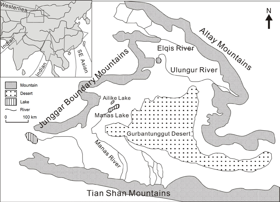
Fig. 1
Map of northern Xinjiang showing the major water systems, including the Manas Lake west of the Gurbantunggut Desert. Inset map shows the northern Xinjiang area (in dotted rectangle) and the present wind systems in Asia (Herzschuh, 2006).
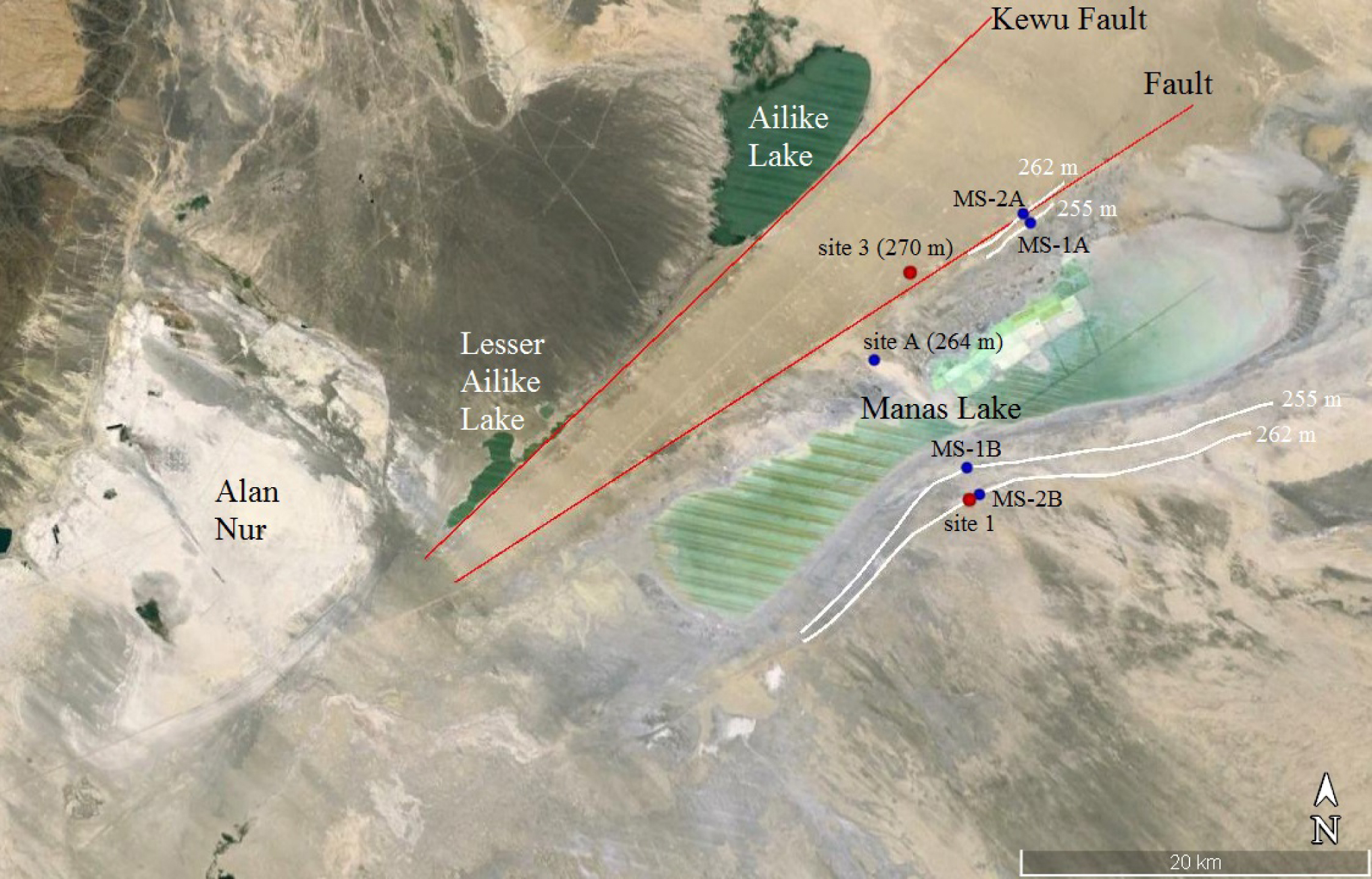
Fig. 2
Google Earth image showing the Manas Lake area and two NE-trending faults. Sampling locations for this study (red dots) and for previous studies by Fan et al. (2012) and Wang (2014) (blue dots) are also shown, together with paleoshorelines (white lines). The elevation shown is in meters above sea level.
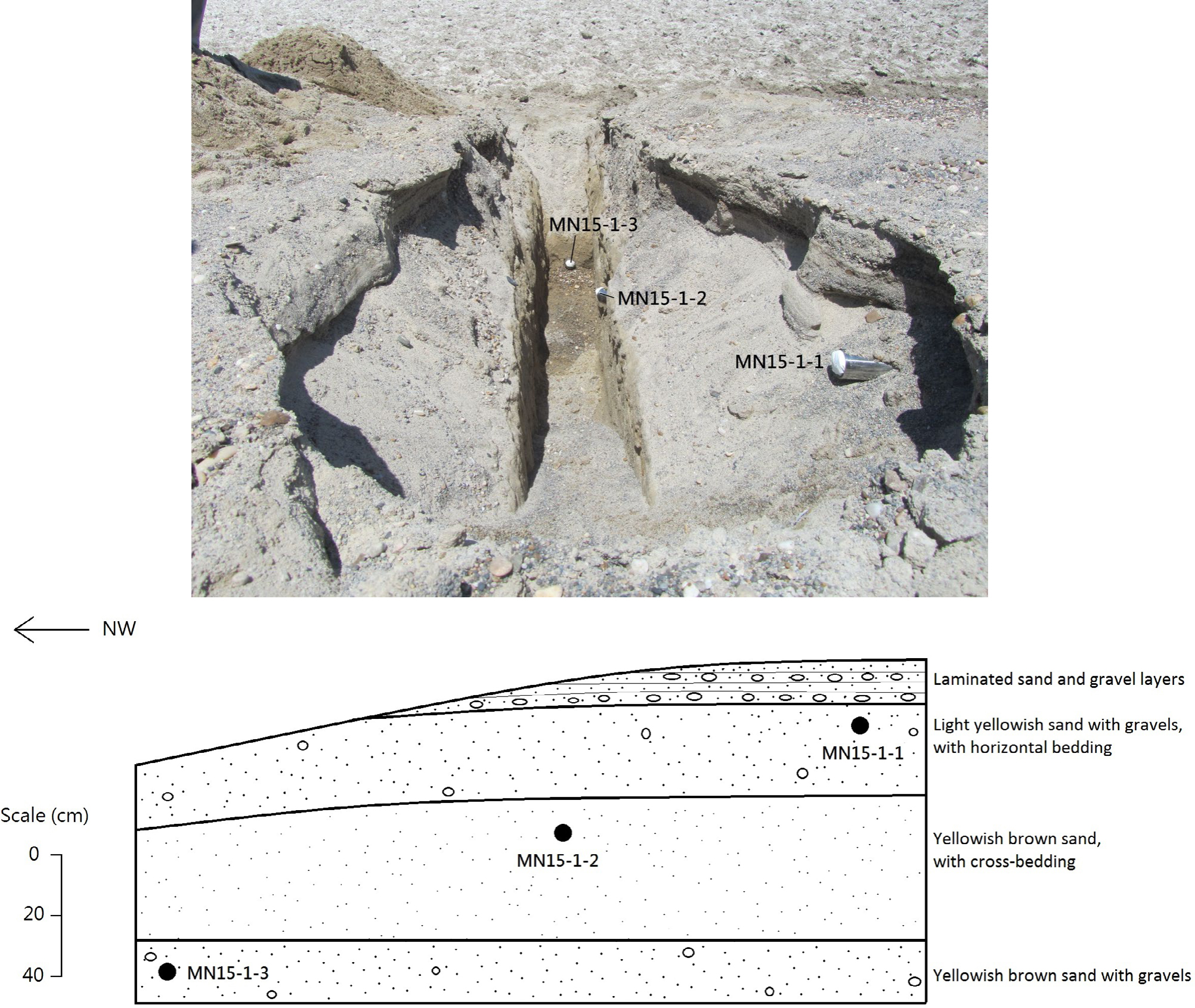
Fig. 3
Field photo showing the excavated trench at paleoshoreline site 1, and the schematic diagram of the section.
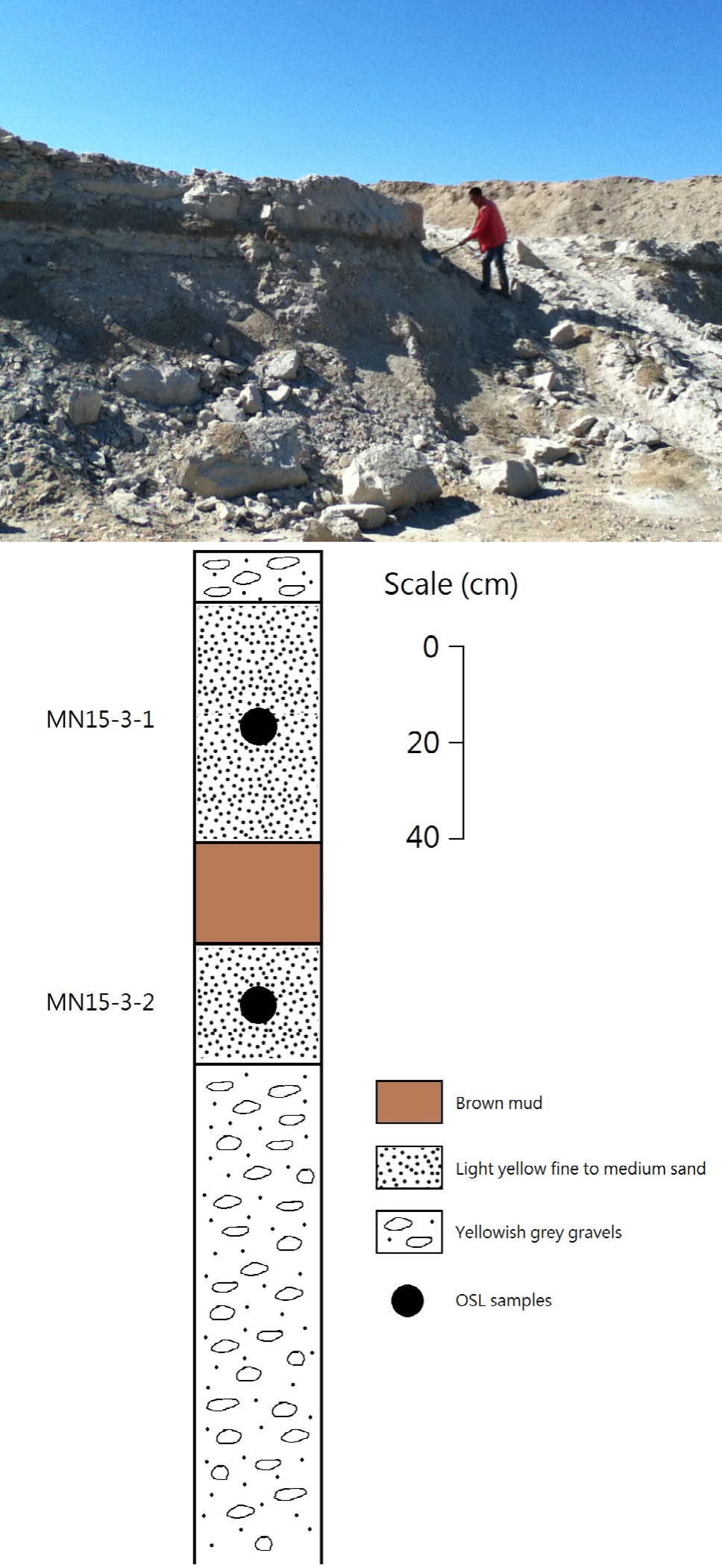
Fig. 4
Field photo and stratigraphic log of the sedimentary section at site 3.
Table 1
The single aliquot regenerative dose (SAR) protocol for quartz post-IR OSL measurements in this study.
| Step | Treatment | Observed |
|---|---|---|
| 1 | Give regenerative dose, Dia | |
| 2 | Preheat at 260°C / 220°Cb for 10 s | |
| 3 | IR stimulation at 125°C for 100 s | |
| 4 | Blue light stimulation at 125°C for 40 s | Lx |
| 5 | Give test dose, DT | |
| 6 | Cut-heat at 220°C / 180°Cb | |
| 7 | IR stimulation at 125°C for 100 s | |
| 8 | Blue light stimulation at 125°C for 40 s | Tx |
| 9 | Blue light bleaching at 280°C for 100 s | |
| 10 | Return to step 1 | |
a For the ‘natural’ sample, i = 0 and D0 = 0. The whole sequence is repeated for several regenerative doses including a zero dose and a repeat dose.
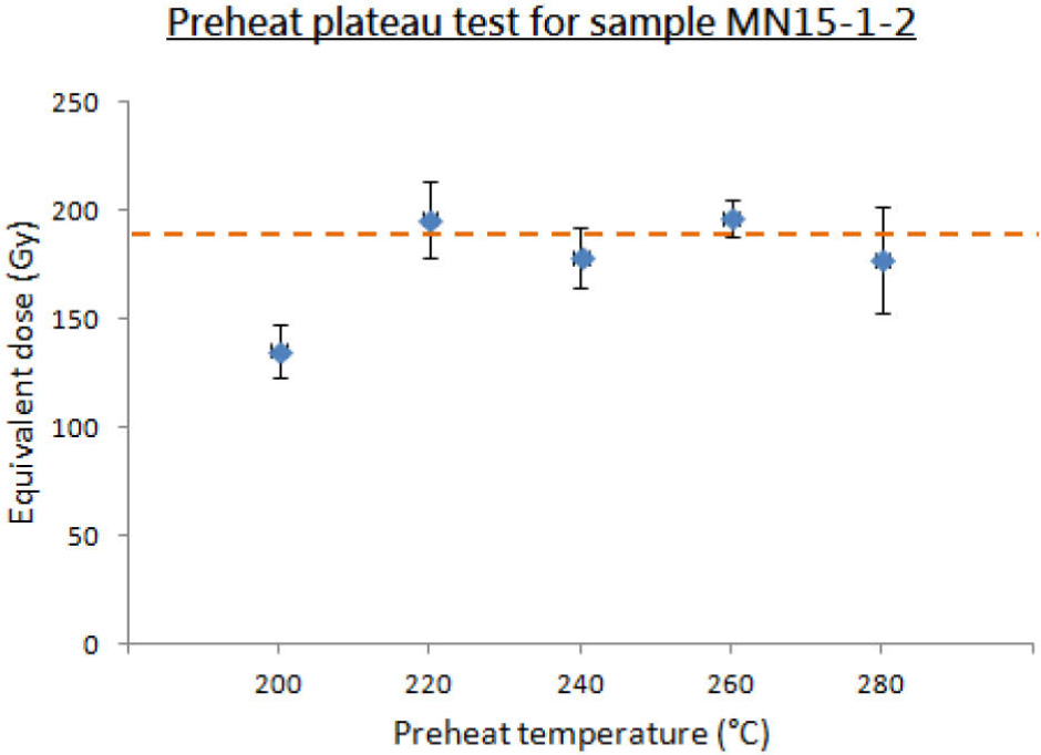
Fig. 5
Preheat plateau test for sample MN15-1-2, with a De plateau obtained for preheat temperatures from 220°C to 280°C.
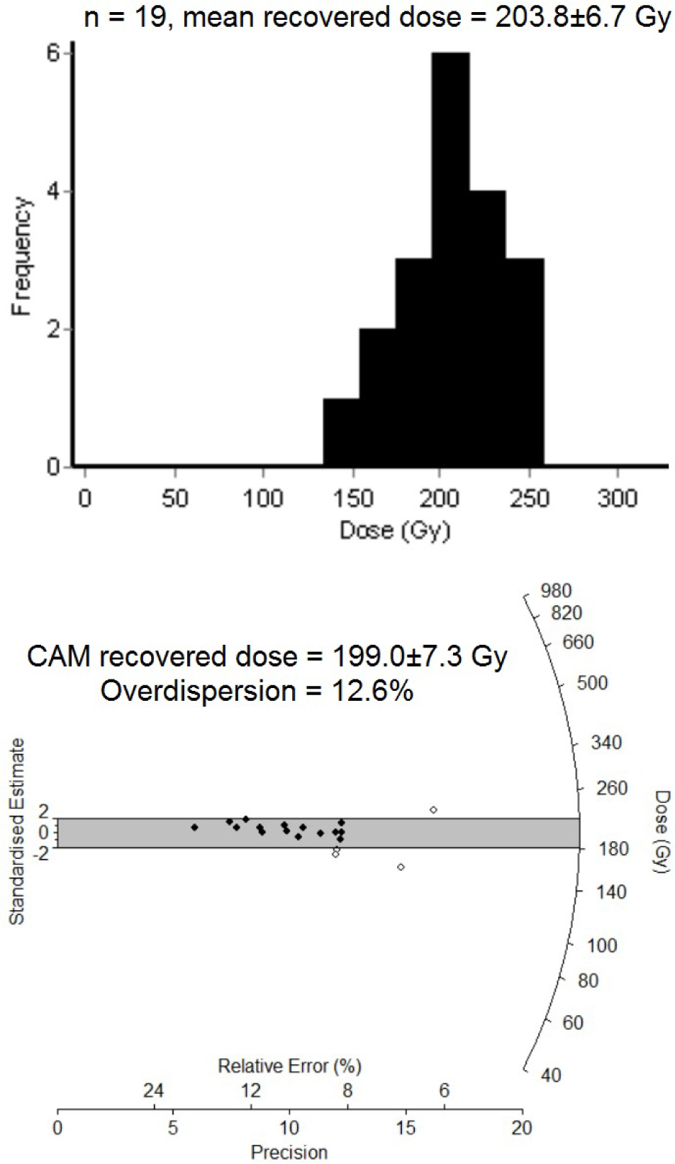
Fig. 6
The distribution of recovered dose values in a dose recovery test of the sample MN15-3-1 is shown using histogram and radial plot. The given laboratory dose was 188 Gy.
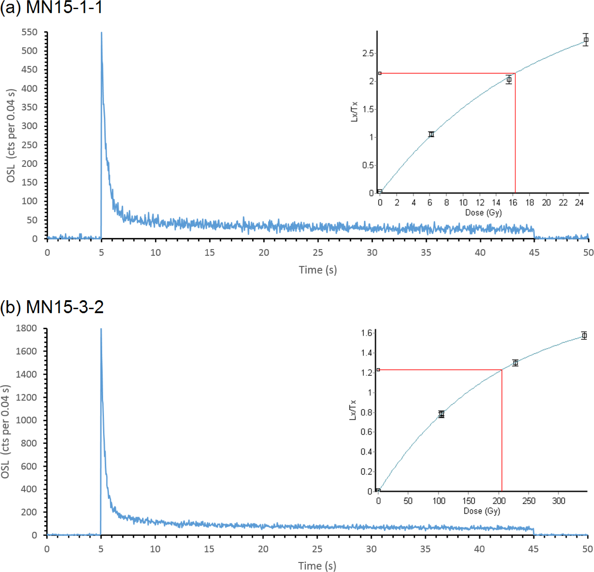
Fig. 7
Typical OSL decay curves and dose response curves (insets) from samples MN15-1-1 and MN15-3-2.
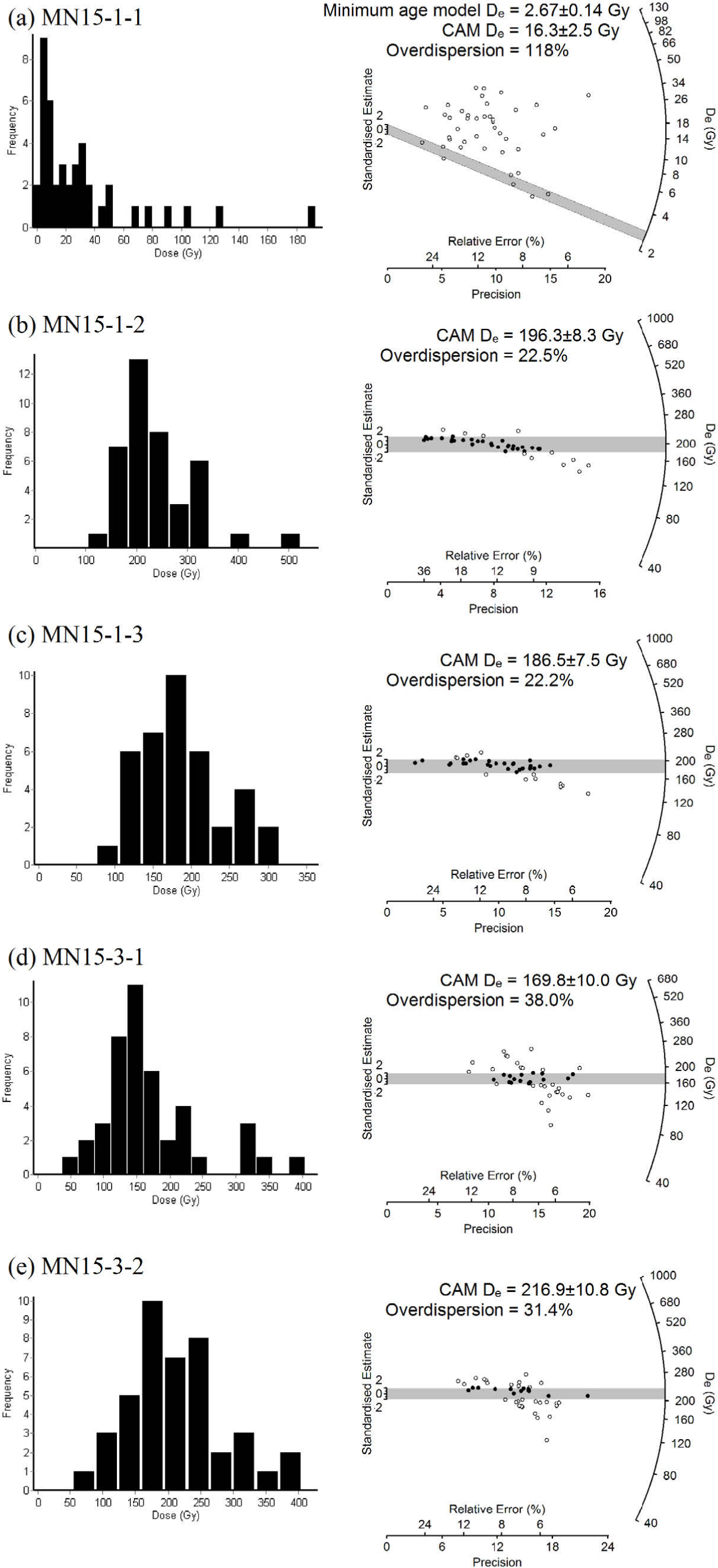
Fig. 8
De distributions of the five samples shown in histograms (left) and radial plots (right).
Table 2
The equivalent doses derived from the mean age model and the central age model, with the overdispersion values for the five samples.
| Sample ID | Number of aliquotsb | Mean age model De (Gy) | Central age model De (Gy) | Over-dispersion(%) |
|---|---|---|---|---|
| MN15-1-1 a | 42 | 31.1 ± 5.9 | 16.3 ± 2.5 | 118 |
| MN15-1-2 | 40 | 219.8 ± 11.7 | 196.3 ± 8.3 | 22.5 |
| MN15-1-3 | 38 | 199.7 ± 8.6 | 186.5 ± 7.5 | 22.2 |
| MN15-3-1 | 43 | 183.9 ± 11.7 | 169.8 ± 10.0 | 38.0 |
| MN15-3-2 | 42 | 229.5 ± 11.2 | 216.9 ± 10.8 | 31.4 |
b 48 aliquots were measured for each sample. Aliquots were rejected by various reasons, including failure in recycling ratio test (4, 4, 4, 2, 2) or recuperation test (2, 1, 1, 1, 0), failure in fitting the dose response curve (0, 0, 0, 0, 2) and when the natural Lx/Tx cannot be interpolated onto the dose response curve (0, 3, 5, 2, 2). The five numbers in brackets refer to the number of aliquots rejected by that specific criteria for the five samples (MN15-1-1, 1-2, 1-3, 3-1, 3-2) respectively.
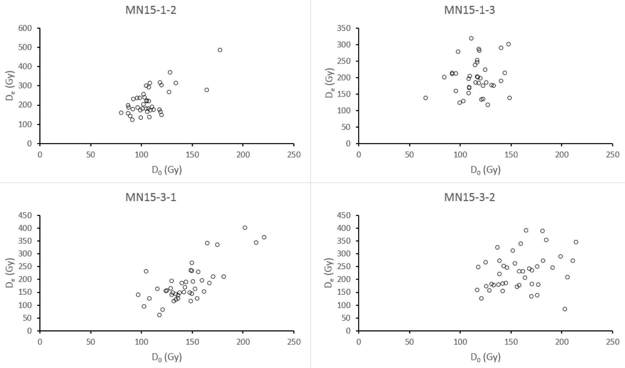
Fig. 9
Plots of De vs D0 for individual aliquots of samples MN15-1-2, MN15-1-3, MN15-3-1 and MN15-3-2.
Table 3
OSL dating results for the five samples in the study area.
| Sampling site | Sample ID | Grain size (µm) | Depth (cm) | α-count rate (cts/ks)a | K content (%)b | Water content (%)c | Cosmic ray (Gy/ka)d | Dose rate (Gy/ka) | Equivalent dose (Gy)e | OSL age (ka)e |
|---|---|---|---|---|---|---|---|---|---|---|
| Site 1 | MN15-1-1 | 180–212 | 22 | 4.97 ± 0.12 | 1.48 | 0.12 | 0.21 | 2.36 ± 0.11 | 2.67 ± 0.14 | 1.13 ± 0.08 |
| MN15-1-2 | 150–180 | 50 | 3.12 ± 0.10 | 1.64 | 1.9 | 0.20 | 2.22 ± 0.13 | 196.3 ± 8.3 | 88.5 ± 6.3 | |
| MN15-1-3 | 150–180 | 70 | 2.82 ± 0.09 | 2.03 | 10.6 | 0.20 | 2.32 ± 0.15 | 186.5 ± 7.5 | 80.3 ± 6.0 | |
| Site 3 | MN15-3-1 | 150–180 | 30 | 4.09 ± 0.12 | 2.20 | 25 | 0.21 | 2.32 ± 0.15 | 169.8 ± 10.0 | 73.3 ± 6.4 |
| MN15-3-2 | 125–150 | 90 | 7.71 ± 0.17 | 2.17 | 25 | 0.19 | 2.71 ± 0.16 | 216.9 ± 10.8 | 80.2 ± 6.1 |
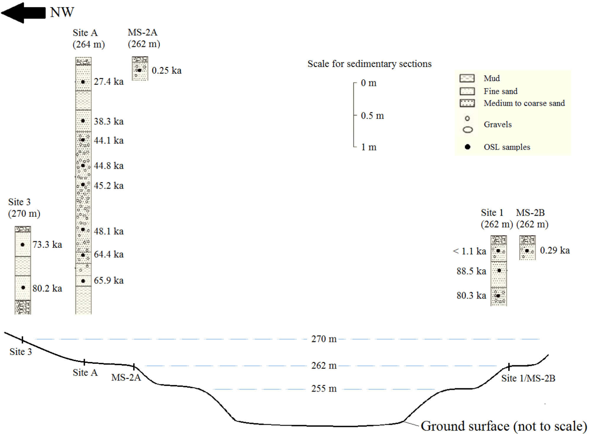
Fig. 10
Summary of results from this studies (sites 1 and 3) and previous studies by Fan et al. (2012) and Wang (2014). Note that the top of each sedimentary section shown corresponds to the ground surface.