
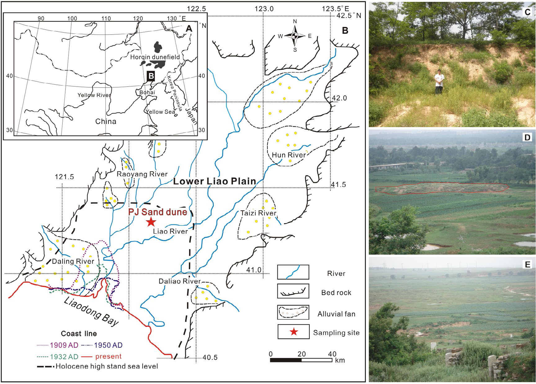
Fig. 1
(A) The location of the study area in NE China. (B) Map showing the geological setting (Lower Liao River plain, local drainage streams and adjacent mountain areas) and coastline changes (sea level in Holocene, coastlines in 1905 AD, 1932 AD, 1950 AD and present, Fu, 1988; Chen et al., 2010). The location of the sampling site is also shown. (C)–(E) Typical sand deposits in the LLP. (C) is a photo of studied PJ sand dune.
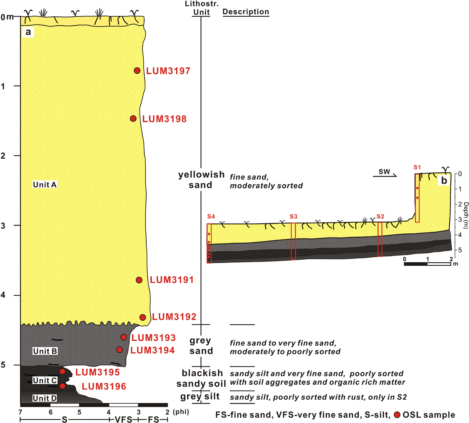
Fig. 2
(A) Investigated profile and its description. The positions of OSL samples are shown in the profile. (B) Stratigraphy of the PJ dune showing the positions of four investigated sections and sampling depths.
Table 1
SAR protocol applied for equivalent dose determination.
| Step | Quartz OSL | K-feldspar post-IR IRSL150 | |||
|---|---|---|---|---|---|
| Treatment | Observed | Step | Treatment | Observed | |
| 1 | Give dose a, Di | 1 | Give dose | ||
| 2 | Preheat for 60 s at 180°C | 2 | Preheat for 60 s at 180°C | ||
| 3 | IR stimulation b for 40 s at 0°C | 3 | IR stimulation for 100 s at 50°C | ||
| 4 | Stimulation for 40 s at 125°C | Ln, Li | 4 | IR stimulation for 200 s at 150°C | Ln, Li |
| 5 | Give test dose, Dt | 5 | Test dose, Dt | ||
| 6 | Heat to 160°C | 6 | Preheat for 60 s at 180°C | ||
| 7 | Stimulate for 40 s at 125°C | Tn, Ti | 7 | IR stimulation for 100 s at 50°C | |
| 8 | Return to 1 | 8 | IR stimulation for 200 s at 150°C Return to 1 | Tn, Ti | |
| 9 | Return to 1 | ||||
Table 2
Dose rate determination
| SampleID | Depth (cm) | Grain size Interval (μm) | U (ppm) | Th (ppm) | K (%) | Water content (%)a | Dose rate(Gy/ka) | |
|---|---|---|---|---|---|---|---|---|
| K-feldspar | quartz | |||||||
| LUM3197 | 80 | 100–150 | 0.96 ± 0.06 | 2.63 ± 0.14 | 2.85 ± 0.14 | 6 ± 4 (1.7) | 4.02 ± 0.17 | 3.24 ± 0.24 |
| LUM3198 | 149 | 100–150 | 1.06 ± 0.06 | 2.82 ± 0.15 | 2.91 ± 0.15 | 6 ± 4 (2.1) | 4.10 ± 0.17 | 3.31 ± 0.24 |
| LUM3191 | 380 | 100–150 | 1.00 ± 0.05 | 2.66 ± 0.14 | 2.79 ± 0.14 | 6 ± 4 (2.6) | 3.96 ± 0.17 | 3.13 ± 0.23 |
| LUM3192 | 434 | 100–150 | 0.91 ± 0.05 | 2.72 ± 0.14 | 2.83 ± 0.14 | 6 ± 4 (4.2) | 3.92 ± 0.16 | 3.15 ± 0.24 |
| LUM3193 | 462 | 100–150 | 1.13 ± 0.06 | 3.27 ± 0.17 | 2.87 ± 0.14 | 6 ± 4 (6.6) | 4.05 ± 0.17 | 3.26 ± 0.24 |
| LUM3194 | 480 | 100–150 | 1.31 ± 0.07 | 4.30 ± 0.22 | 2.82 ± 014 | 6 ± 4 (9.5) | 4.12 ± 0.17 | 3.32 ± 0.24 |
| LUM3195 | 511 | 63–100 | 1.88 ± 0.10 | 6.95 ± 0.35 | 2.61 ± 0.13 | 13 ± 3 (14) | 4.14 ± 0.17 | 3.20 ± 0.22 |
| LUM3196 | 532 | 63–100 | 2.24 ± 0.12 | 8.01 ± 0.41 | 2.34 ± 0.12 | 13 ± 3 (15) | 4.07 ± 0.17 | 3.10 ± 0.20 |
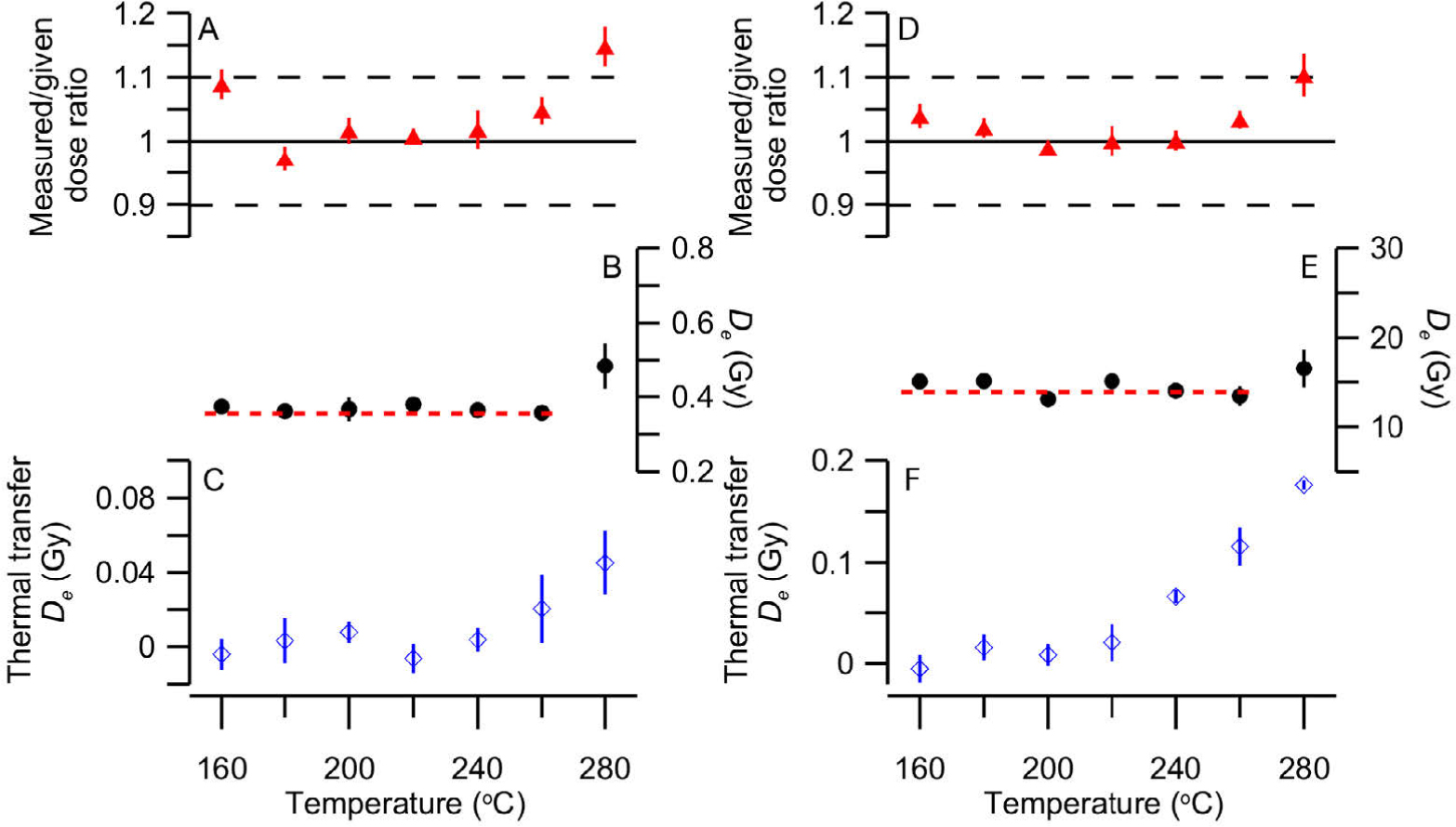
Fig. 3
Results of quartz OSL pre-tests. (A) Measured/given ratio (dose recovery test), (B) equivalent dose and (C) thermal transfer at different preheat temperatures for sample LUM3192. (D)–(F) show the results of the same set of tests for sample LUM3196.
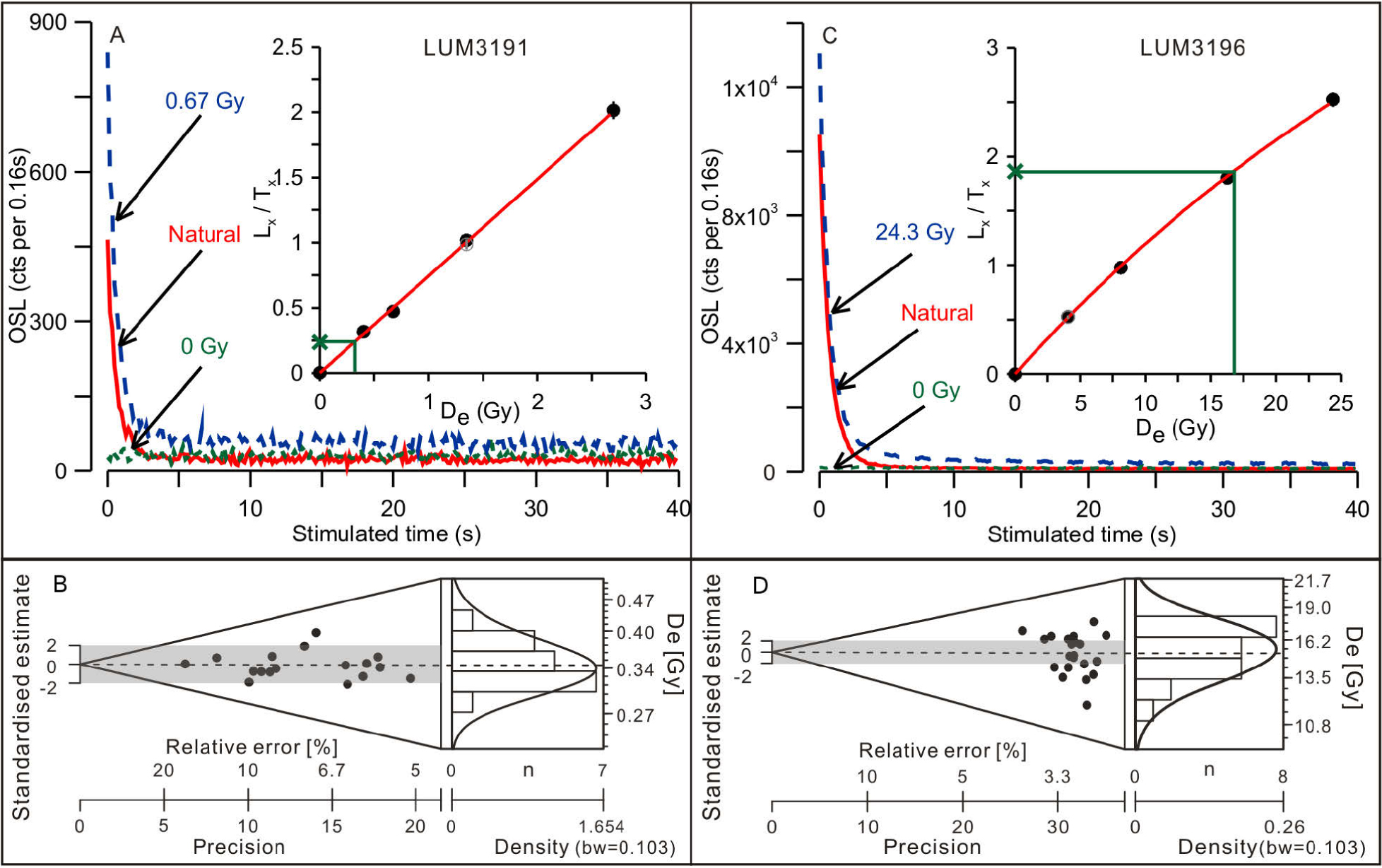
Fig. 4
Quartz decay curve, dose response curve and De distribution for sample LUM3191–(A) and (B); for sample LUM3196–(C) and (D). De distributions are presented using abanico plots (Dietze et al., 2016).
Table 3
Result of OSL dating
| Feldspar | ||||||||||||||
|---|---|---|---|---|---|---|---|---|---|---|---|---|---|---|
| LumNo. | Depth (cm) | Quartz | pIRIR150 | IR50 | ||||||||||
| (cm) Dose rate (Gy/ka) | De (Gy) | Age (a) | σOD (%)a | Dose rate (Gy/ka) | De (Gy) | g2days (%/decade) | Age (a) | Corrected age (a) | De (Gy) | g2days (%/decade) | Age (a) | Corrected age (a) | ||
| 3197 | 80 | 3.24±0.23 | 0.28±0.01 | 87±7 | 6.3 | 4.02±0.17 | 0.81±0.05 | 0.99±0.38 | 202±15 | 214±21 | 0.34±0.01 | 8.38±0.59 | 85±4 | 145±13 |
| 3198 | 149 | 3.31±0.24 | 0.28±0.01 | 85±7 | 4.4 | 4.10±0.17 | 0.88±0.06 | 1.96±0.41 | 215±18 | 243±26 | 0.35±0.01 | 9.23±0.64 | 86±5 | 159±18 |
| 3191 | 380 | 3.13±0.23 | 0.34±0.01 | 110±9 | 6.6 | 3.96±0.17 | 0.68±0.03 | 0.38±0.28 | 173±10 | 177±14 | 0.38±0.01 | 9.18±0.52 | 96±5 | 178±17 |
| 3192 | 434 | 3.15±0.23 | 0.36±0.01 | 115±9 | 5.9 | 3.92±0.16 | 0.74±0.03 | 1.11±0.39 | 189±12 | 203±17 | 0.39±0.01 | 9.30±0.54 | 100±4 | 187±17 |
| 3193 | 462 | 3.26±0.24 | 0.37±0.01 | 114±9 | 12.5 | 4.05±0.17 | 0.66±0.03 | 0.44±0.31 | 164±9 | 168±13 | 0.39±0.01 | 9.36±0.74 | 96±5 | 181±21 |
| 3194 | 480 | 3.31±0.24 | 0.42±0.01 | 128±10 | 6.7 | 4.12±0.17 | 0.60±0.05 | 0.62±0.42 | 145±13 | 151±17 | 0.46±0.03 | 7.80±0.74 | 111±8 | 186±25 |
| 3195 | 511 | 3.19±0.22 | 4.69±0.14 | 1470±110 | 12.3 | 4.14±0.17 | 5.77±0.24 | 0.25±0.41 | 1390±80 | 1430±120 | 4.28±0.18 | 4.99±0.26 | 1040±60 | 1500±120 |
| 3196 | 532 | 3.08±0.21 | 15.3±0.3 | 4970±350 | 10.1 | 4.07±0.17 | 22.1±1.7 | 0.80±0.28 | 5420±470 | 5760±620 | 14.1±0.4 | 4.45±0.19 | 3480±180 | 4950±350 |
a σOD values were calculated according to Galbraith et al. (1999).
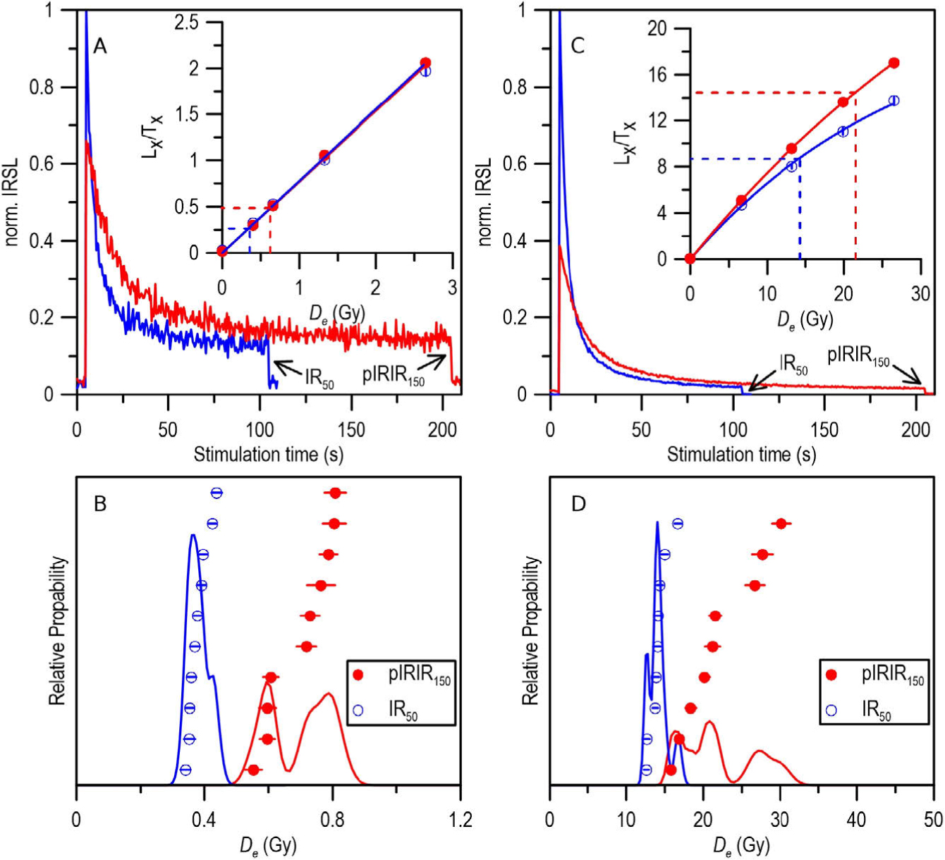
Fig. 5
K-feldspar IR50 and pIRIR150 decay curve, growth curve and De distribution for sample LUM3191–(A) and (B), for sample LUM3196–(C) and (D).
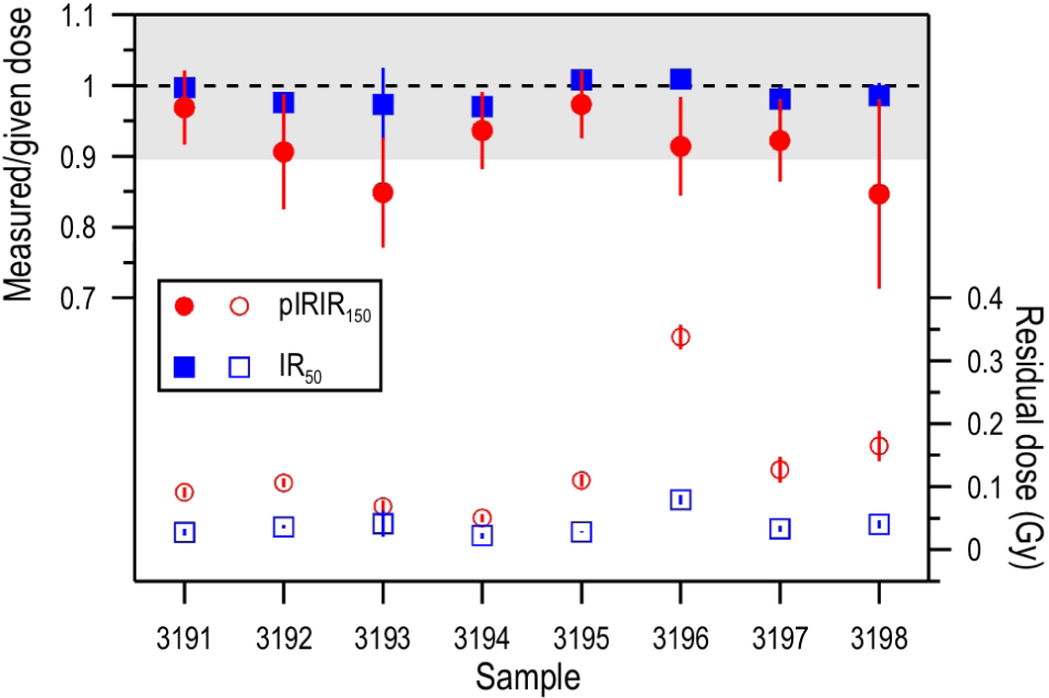
Fig. 6
Dose recovery ratio and residual dose for IR50 and pIRIR150 for each sample.
Table 4
Summary of predicted residual dose and measured residual dose (4 h SOL2 bleaching).
| Sample | pIRIR150 | IR50 | ||
|---|---|---|---|---|
| Predicted | Measured | Predicted | Measured | |
| residual | residual | residual | residual | |
| 3197 | 0.48 ± 0.07 | 0.13 ± 0.02 | 0.00 ± 0.06 | 0.03 ± 0.00 |
| 3198 | 0.57 ± 0.08 | 0.16 ± 0.02 | 0.14 ± 0.06 | 0.04 ± 0.01 |
| 3191 | 0.26 ± 0.06 | 0.09 ± 0.01 | 0.12 ± 0.05 | 0.03 ± 0.01 |
| 3192 | 0.32 ± 0.06 | 0.11 ± 0.01 | 0.12 ± 0.04 | 0.04 ± 0.00 |
| 3193 | 0.21 ± 0.06 | 0.07 ± 0.01 | 0.11 ± 0.05 | 0.04 ± 0.02 |
| 3194 | 0.09 ± 0.09 | 0.05 ± 0.01 | 0.12 ± 0.07 | 0.02 ± 0.00 |
| 3195 | -0.19 ± 0.06 | 0.11 ± 0.01 | -0.18 ± 0.06 | 0.03 ± 0.00 |
| 3196 | 2.91 ± 0.09 | 0.34 ± 0.02 | 0.87 ± 0.05 | 0.08 ± 0.01 |
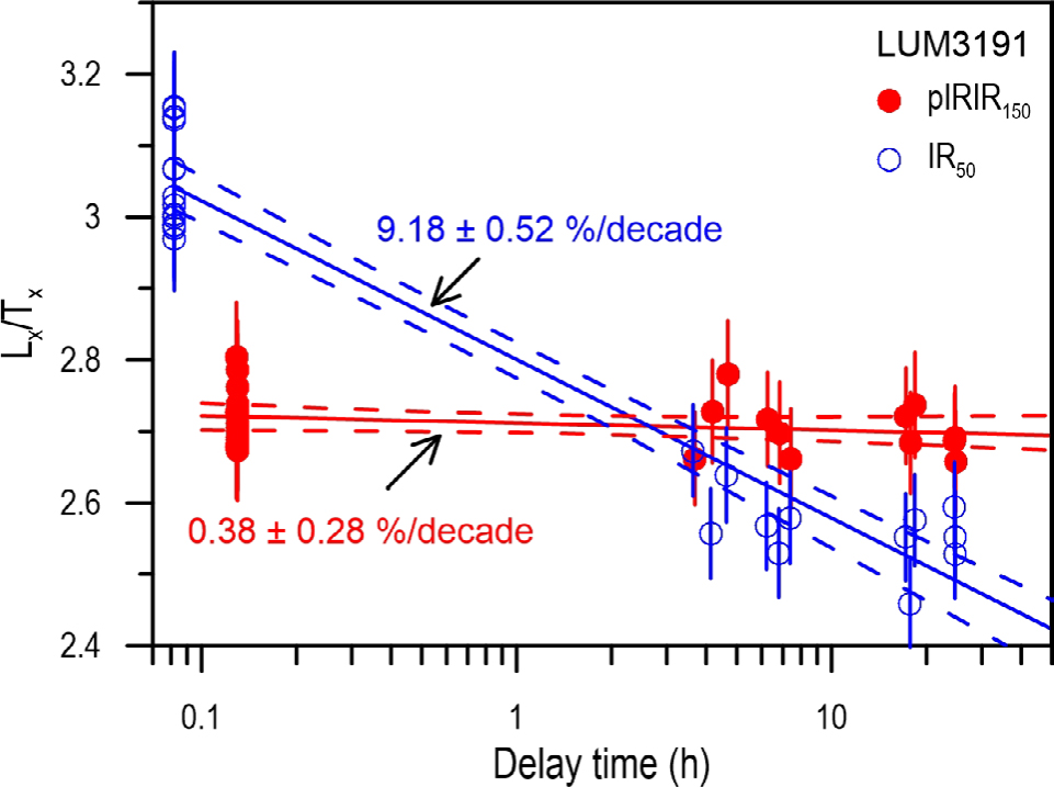
Fig. 7
Fading rate (g2ays-value) of IR50 and pIRIR150 signals for one representative sample LUM3191.
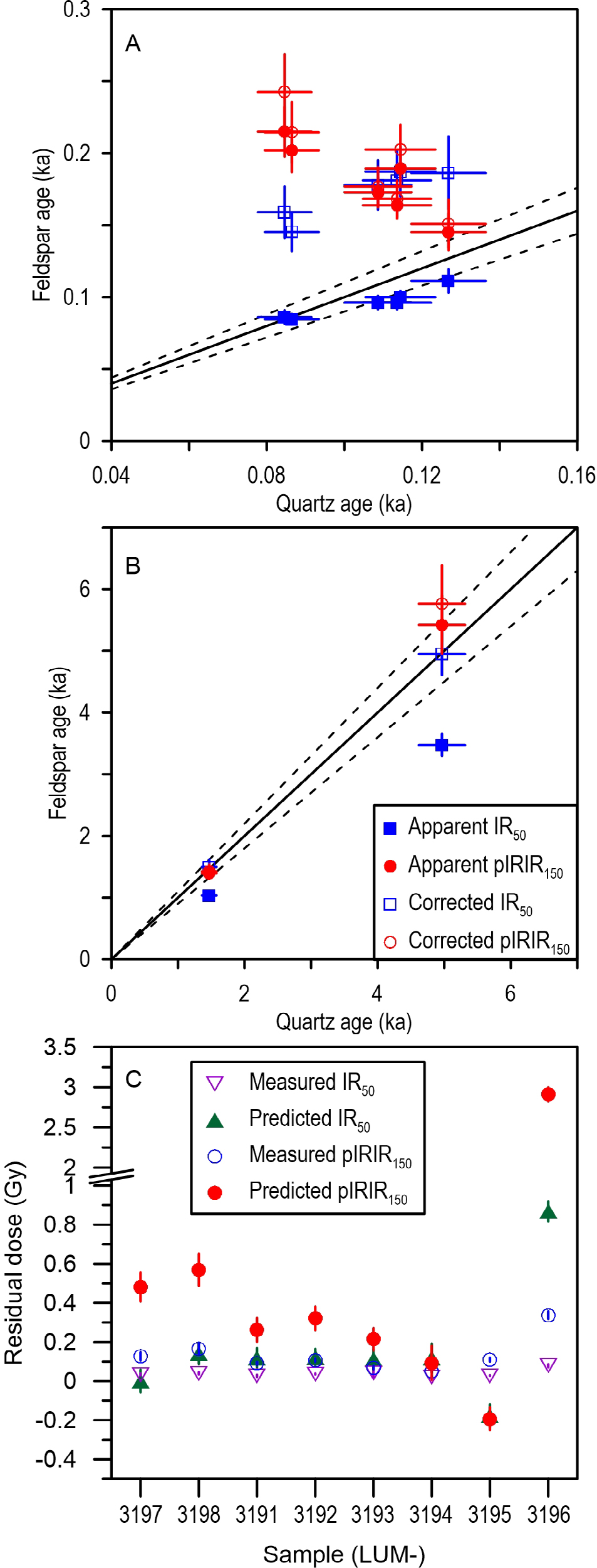
Fig. 8
Ages from different luminescence signals and the comparison of the predicted and measured residual doses. A shows the comparison for the sand samples, B shows the comparison for two sandy soil samples. C demonstrates the comparison of the predicted residual dose and measured dose for all samples (See details in text).
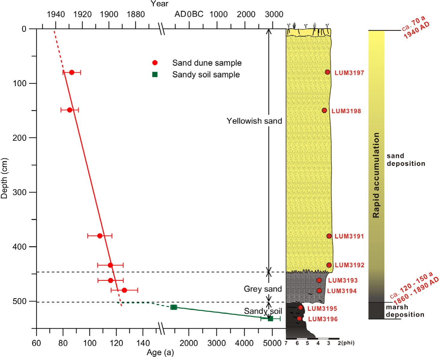
Fig. 9
Depth-age relationship of the PJ sand dune and sandy soil layer with a graphic log and all sample codes.
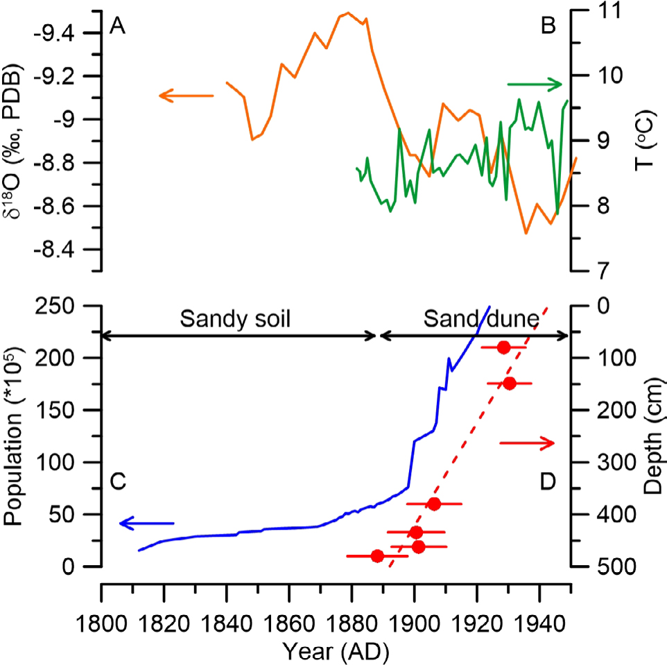
Fig. 10
Comparison of different proxies. (A) The precipitation variations in northern China revealed by the δ18O data from the Shihua Cave stalagmites record (Li et al., 1998; orange solid line). (B) Temperature change in Liaoning Province (Sun and Zhao, 2002; green solid line). (C) Population change in Northeastern China from 1812 to 1911 AD (blue solid line) summarized by Zhao (2004). (D) Quartz OSL ages for the sand deposits.