

Tab. 1
The descriptive statistics of the considered assets
| In-sample | Out-of-sample | |||||||||||
|---|---|---|---|---|---|---|---|---|---|---|---|---|
| SPX | DAX | AAPL | MSFT | HGF | CBF | SPX | DAX | AAPL | MSFT | HGF | CBF | |
| %ARC | 3.92 | 4.79 | 35.22 | 6.32 | 9.41 | 12.14 | 9.67 | 8.07 | 22.68 | 25.70 | -0.62 | -11.01 |
| %ASD | 20.39 | 24.97 | 46.69 | 33.06 | 28.48 | 34.54 | 11.94 | 18.37 | 22.27 | 21.43 | 19.25 | 33.07 |
| IR | 0.19 | 0.19 | 0.75 | 0.19 | 0.33 | 0.35 | 0.81 | 0.44 | 1.02 | 1.2 | -0.03 | -0.33 |
| %MDD | 56.78 | 72.68 | 43.80 | 71.65 | 68.37 | 73.48 | 14.16 | 29.27 | 30.45 | 18.05 | 42.47 | 75.83 |
[i] %ARC - annualized rate of return (%), %ASD - annualized standard deviation (%), %MDD - maximum drawdown of capital (%), IR - information ratio calculated as %ARC / %ASD, OC - optimization criterion calculated as 100 * (%ARC * %ARC) / (%ASD * %MDD), SPX - S&P500 Index, DAX - Deutscher Aktienindex, AAPL - Apple Inc. stock, MSFT - Microsoft Corp. stock, HGF - High Grade Copper Futures, CBF - Crude Oil Brent Futures. The statistics have been calculated for in-sample period from the beginning of 1998 to the end of 2013 and for out-of-sample period from the beginning of 2013 to the end of 2017, on daily data.
Tab. 2
The median strategies parameters and statistics resulted from all the methods for SPXDAX
| In-sample | Out-of-sample | |||||||
|---|---|---|---|---|---|---|---|---|
| ES | EHC | GM | DEM | ES | EHC | GM | DEM | |
| k1 | 60.00 | 100.00 | 100.00 | 100.00 | 60.00 | 100.00 | 100.00 | 100.00 |
| k2 | 45.00 | 35.00 | 35.00 | 35.00 | 45.00 | 35.00 | 35.00 | 35.00 |
| k1.2 | 65.00 | 45.00 | 45.00 | 45.00 | 65.00 | 45.00 | 45.00 | 45.00 |
| k2.2 | 75.00 | 85.00 | 85.00 | 85.00 | 75.00 | 85.00 | 85.00 | 85.00 |
| %ARC | 4.27 | 3.92 | 3.92 | 3.92 | -0.03 | -0.62 | -0.62 | -0.62 |
| %ASD | 5.17 | 4.63 | 4.63 | 4.63 | 4.02 | 3.74 | 3.74 | 3.74 |
| IR | 0.83 | 0.85 | 0.85 | 0.85 | -0.01 | -0.17 | -0.17 | -0.17 |
| %MDD | 4.53 | 4.30 | 4.30 | 4.30 | 7.20 | 6.34 | 6.34 | 6.34 |
| OC | 77.79 | 77.16 | 77.16 | 77.16 | 0.00 | -1.62 | -1.62 | -1.62 |
[i] %ARC - annualized rate of return (%), %ASD - annualized standard deviation (%), %MDD - maximum drawdown of capital (%), IR - information ratio calculated as %ARC / %ASD, OC - optimization criterion calculated as 100 * (%ARC * %ARC) / (%ASD * %MDD), k1, k2, k1.2, k2.2 - strategy parameters, width of the moving averages’ windows. The statistics of the equity lines have been calculated for the strategy working on daily frequency, investing 20% of capital in position on each asset with rebalancing every 5 trading days. Trading from the beginning of 1998 to the end of 2013 has been simulated, with the assumption of fee equal to 0.25% of the position value.
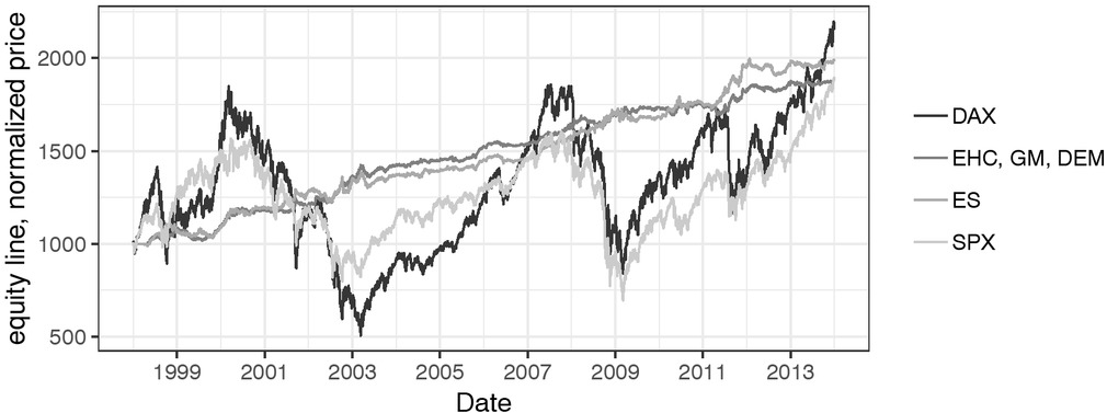
Fig. 1
The equity lines of the strategies selected by all the methods for SPXDAX - in-sample
SPX - S&P500 Index, DAX - Deutscher Aktienindex, ES, EHC, GD, DEM - equity line of the median strategy resulted from respectively Exhaustive Search, Extended Hill Climbing, Grid Method and Differential Evolution Method. Prices of both assets have been normalized in order to have initial value equal to 1000. The equity line has been calculated for the strategy working on daily frequency, investing 20% of capital in position on each asset with rebalancing every 5 trading days. Trading from the beginning of 1998 to the end of 2013 has been simulated, with the assumption of fee equal to 0.25% of the position value.
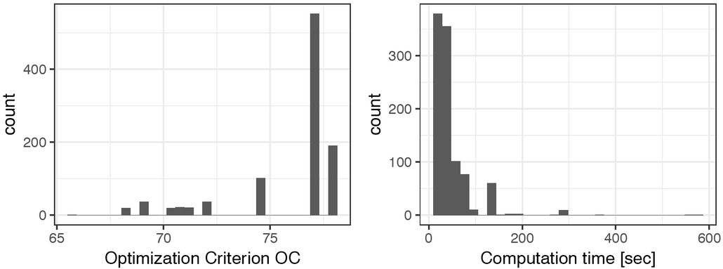
Fig. 2
The histograms of the reached optimization criterion and the execution time of EHC for SPXDAX – in-sample
OC - optimization criterion calculated as 100 * (%ARC * %ARC) / (%ASD * %MDD). The optimization criterion have been calculated from the sample of 1000 independent algorithm executions. The strategies have been working on the daily frequency, investing 20% of capital in position on each asset with rebalancing every 5 trading days. Trading from the beginning of 1998 to the end of 2013 has been simulated, with assumption of fee equal to 0.25% of the position value.
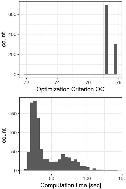
Fig. 3
The histograms of the reached optimization criterion and the execution time of DEM for SPXDAX - in-sample
OC - optimization criterion calculated as 100 * (%ARC * %ARC) / (%ASD * %MDD). The equity lines have been calculated for the strategy working on daily frequency, investing 20% of capital in position on each asset with rebalancing every 5 trading days. Trading from the beginning of 1998 to the end of 2013 has been simulated, with the assumption of fee equal to 0.25% of the position value.
Tab. 3
The summary of the reached optimization criterion and the execution time of methods for SPXDAX – in-sample
| ES | EHC | GM | DEM | |||||
|---|---|---|---|---|---|---|---|---|
| OC | Time [sec] | OC | Time [sec] | OC | Time [sec] | OC | Time [sec] | |
| Minimum | 77.79 | 35562.17 | 65.58 | 11.87 | 77.16 | 128.04 | 71.93 | 13.11 |
| 1st Quantile | 77.79 | 35562.17 | 74.39 | 13.93 | 77.16 | 128.04 | 77.16 | 24.84 |
| Median | 77.79 | 35562.17 | 77.16 | 30.97 | 77.16 | 128.04 | 77.16 | 31.15 |
| Mean | 77.79 | 35562.17 | 75.94 | 43.1 | 77.16 | 128.04 | 77.34 | 42.73 |
| 2nd Quantile | 77.79 | 35562.17 | 77.16 | 65.32 | 77.16 | 128.04 | 77.79 | 61.5 |
| Max | 77.79 | 35562.17 | 77.79 | 569.39 | 77.16 | 128.04 | 77.79 | 141.08 |
| Standard deviation | 0.00 | 0.00 | 2.61 | 48.77 | 0.00 | 0.00 | 0.36 | 24.06 |
[i] OC - optimization criterion calculated as 100 * (%ARC * %ARC) / (%ASD * %MDD). The optimization criterion have been calculated for the strategy working on daily frequency, investing 20% of the capital in position on each asset with rebalancing every 5 trading days. Trading from the beginning of 1998 to the end of 2013 has been simulated, with the assumption of fee equal to 0.25% of the position value.
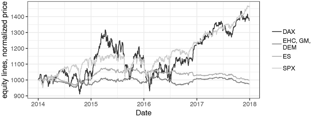
Fig. 4
The equity lines of the strategies selected by the all the methods for SPXDAX – out-of-sample
ES, EHC, GD, DEM - equity line of the median strategy resulted from respectively Exhaustive Search, Extended Hill Climbing, Grid Method and Differential Evolution Method. Prices of both assets have been normalized in order to have initial value equal to 1000. The equity line has been calculated for the strategy working on daily frequency, investing 20% of capital in position on each asset with rebalancing every 5 trading days. Trading from the beginning of 2014 to the end of 2017 has been simulated, with the assumption of fee equal to 0.25% of the position value.
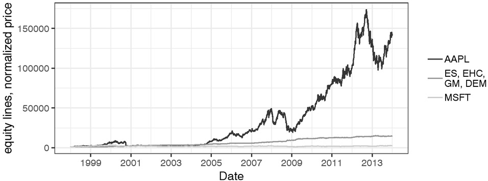
Fig. 5
The equity line of the strategy selected by all the methods for AAPLMSFT – in-sample
AAPL - Apple Inc. stock, MSFT - Microsoft Corp. stock, ES, EHC, GD, DEM - equity line of the median strategy resulted from respectively Exhaustive Search, Extended Hill Climbing, Grid Method and Differential Evolution Method. Prices of both assets have been normalized in order to have initial value equal to 1000. The equity line has been calculated for the strategy working on daily frequency, investing 20% of capital in position on each asset with rebalancing every 5 trading days. Trading from the beginning of 1998 to the end of 2013 has been simulated, with the assumption of fee equal to 0.25% of the position value.
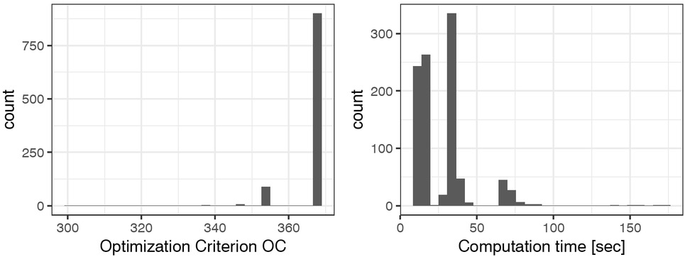
Fig. 6
The histograms of the reached optimization criterion and the execution time of EHC for AAPLMSFT – in-sample
OC - optimization criterion calculated as 100 * (%ARC * %ARC) / (%ASD * %MDD). The optimization criterion has been calculated from the sample of 1000 independent algorithm executions. The strategies have been working on the daily frequency, investing 20% of capital in position on each asset with rebalancing every 5 trading days. Trading from the beginning of 1998 to the end of 2013 has been simulated, with the assumption of fee equal to 0.25% of the position value.
Tab. 4
The median strategy parameters and statistics resulted from all the methods for AAPLMSFT
| In-sample | Out-of-sample | |||||||
|---|---|---|---|---|---|---|---|---|
| ES | EHC | GM | DEM | ES | EHC | GM | DEM | |
| k1 | 50.00 | 50.00 | 50.00 | 50.00 | 50.00 | 50.00 | 50.00 | 50.00 |
| k2 | 60.00 | 60.00 | 60.00 | 60.00 | 60.00 | 60.00 | 60.00 | 60.00 |
| k1.2 | 75.00 | 75.00 | 75.00 | 75.00 | 75.00 | 75.00 | 75.00 | 75.00 |
| k2.2 | 40.00 | 40.00 | 40.00 | 40.00 | 40.00 | 40.00 | 40.00 | 40.00 |
| %ARC | 17.79 | 17.79 | 17.79 | 17.79 | 1.37 | 1.37 | 1.37 | 1.37 |
| %ASD | 11.13 | 11.13 | 11.13 | 11.13 | 5.68 | 5.68 | 5.68 | 5.68 |
| IR | 1.60 | 1.60 | 1.60 | 1.60 | 0.24 | 0.24 | 0.24 | 0.24 |
| %MDD | 7.71 | 7.71 | 7.71 | 7.71 | 9.54 | 9.54 | 9.54 | 9.54 |
| OC | 368.83 | 368.83 | 368.83 | 368.83 | 3.49 | 3.49 | 3.49 | 3.49 |
[i] %ARC - annualized rate of return (%), %ASD - annualized standard deviation (%), %MDD - maximum drawdown of capital (%), IR - information ratio calculated as %ARC / %ASD, OC - optimization criterion calculated as 100 * (%ARC * %ARC) / (%ASD * %MDD), k1, k2, k1.2, k2.2 - strategy parameters, width of the moving averages’ windows. The statistics of the equity line have been calculated for the strategy working on daily frequency, investing 20% of capital in position on each asset with rebalancing every 5 trading days. Trading from the beginning of 1998 to the end of 2013 has been simulated, with the assumption of fee equal to 0.25% of the position value.
Tab. 5
The summary of the reached optimization criterion and the execution time of methods for AAPLMSFT – in-sample
| ES | EHC | GM | DEM | |||||
|---|---|---|---|---|---|---|---|---|
| OC | Time [sec] | OC | Time [sec] | OC | Time [sec] | OC | Time [sec] | |
| Minimum | 368.83 | 32821.18 | 301.34 | 11.96 | 368.83 | 150.66 | 274.97 | 11.82 |
| 1st Quantile | 368.83 | 32821.18 | 368.83 | 14 | 368.83 | 150.66 | 368.83 | 19.67 |
| Median | 368.83 | 32821.18 | 368.83 | 18.18 | 368.83 | 150.66 | 368.83 | 22.19 |
| Mean | 368.83 | 32821.18 | 367.16 | 27.4 | 368.83 | 150.66 | 368.55 | 22.71 |
| 2nd Quantile | 368.83 | 32821.18 | 368.83 | 32.97 | 368.83 | 150.66 | 368.83 | 25.27 |
| Max | 368.83 | 32821.18 | 368.83 | 174.06 | 368.83 | 150.66 | 368.83 | 45.8 |
| Standard deviation | 0.00 | 0.00 | 5.51 | 18.71 | 0.00 | 0.00 | 5.14 | 4.52 |
[i] OC - optimization criterion calculated as 100 * (%ARC * %ARC) / (%ASD * %MDD). The optimization criterion has been calculated from the sample of 1000 independent algorithm executions. The strategies have been working on the daily frequency, investing 20% of capital in position on each asset with rebalancing every 5 trading days. Trading from the beginning of 1998 to the end of 2013 has been simulated, with the assumption of fee equal to 0.25% of the position value.
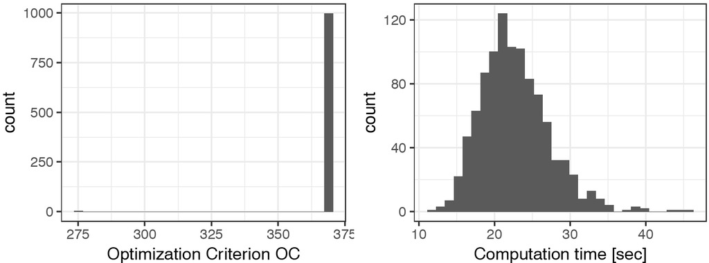
Fig. 7
The histograms of the reached optimization criterion and the execution time of DEM for AAPLMSFT – in-sample OC - optimization criterion calculated as 100 * (%ARC * %ARC) / (%ASD * %MDD). The optimization criterion have been calculated from the sample of 1000 independent algorithm executions. The strategies have been working on the daily frequency, investing 20% of capital in position on each asset with rebalancing every 5 trading days. Trading from the beginning of 1998 to the end of 2013 has been simulated, with the assumption of fee equal to 0.25% of the position value.
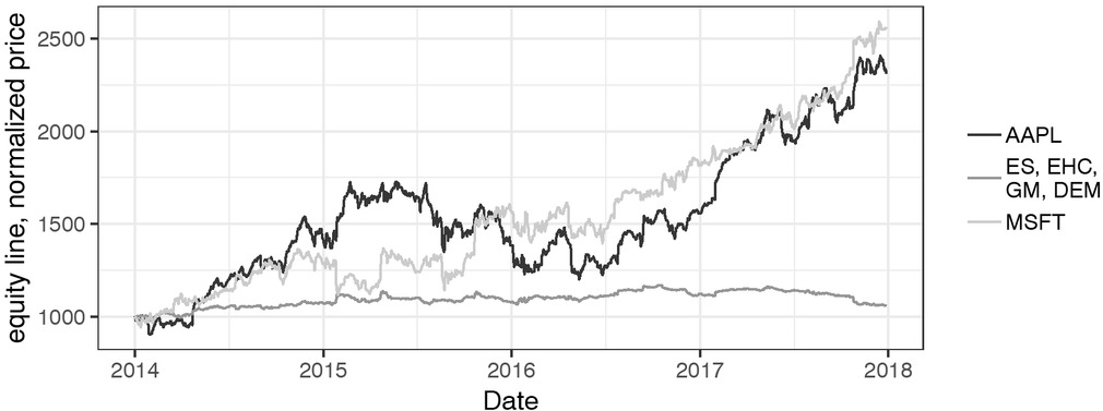
Fig. 8
The equity lines of the strategies selected by all the methods for AAPLMSFT – out-of-sample
AAPL - Apple Inc. stock, MSFT - Microsoft Corp. stock, ES, EHC, GD, DEM - equity line of the median strategy resulted from respectively Exhaustive Search, Extended Hill Climbing, Grid Method and Differential Evolution Method. Prices of both assets have been normalized in order to have initial value equal to 1000. The equity line has been calculated for the strategy working on daily frequency, investing 20% of capital in position on each asset with rebalancing every 5 trading days. Trading from the beginning of 2014 to the end of 2017 has been simulated, with the assumption of fee equal to 0.25% of the position value.
Tab. 6
The median strategies parameters and statistics resulted from all the methods for HGFCBF
| In-sample | Out-of-sample | |||||||
|---|---|---|---|---|---|---|---|---|
| k1 | ES 60.00 | EHC 60.00 | GM 60.00 | DEM 60.00 | ES 60.00 | EHC 60.00 | GM 60.00 | DEM 60.00 |
| k2 | 75.00 | 75.00 | 75.00 | 75.00 | 75.00 | 75.00 | 75.00 | 75.00 |
| k1.2 | 50.00 | 30.00 | 30.00 | 30.00 | 50.00 | 30.00 | 30.00 | 30.00 |
| k2.2 | 25.00 | 95.00 | 95.00 | 95.00 | 25.00 | 95.00 | 95.00 | 95.00 |
| %ARC | 8.18 | 9.53 | 9.53 | 9.53 | -1.59 | 6.60 | 6.60 | 7.38 |
| %ASD | 8.16 | 9.83 | 9.83 | 9.83 | 7.09 | 8.17 | 8.17 | 8.07 |
| IR | 1.00 | 0.97 | 0.97 | 0.97 | -0.22 | 0.81 | 0.81 | 0.91 |
| %MDD | 7.51 | 9.52 | 9.52 | 9.52 | 15.86 | 12.16 | 12.16 | 12.16 |
| OC | 109.11 | 97.04 | 97.04 | 97.04 | -2.24 | 43.81 | 43.81 | 55.49 |
[i] OC - optimization criterion calculated as 100 * (%ARC * %ARC) / (%ASD * %MDD). The empirical statistics have been calculated from the sample of 1000 independent algorithm executions. The strategies have been working on the daily frequency, investing 20% of capital in position on each asset with rebalancing every 5 trading days. Trading from the beginning of 1998 to the end of 2013 has been simulated, with the assumption of fee equal to 0.25% of the position value.
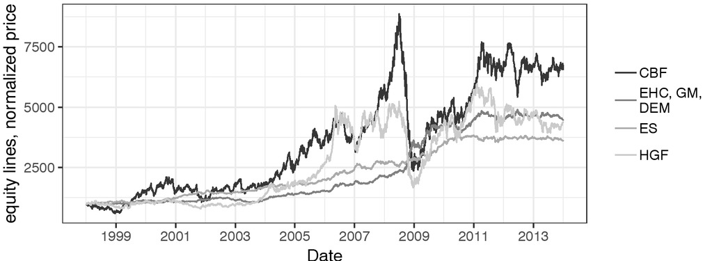
Fig. 9
The equity lines of the strategy selected by all the methods for HGFCBF – in-sample
HGF - High Grade Copper Futures, CBF - Crude Oil Brent Futures, ES, EHC, GD, DEM - equity line of the median strategy resulted from respectively Exhaustive Search, Extended Hill Climbing, Grid Method and Differential Evolution Method. Prices of the both assets have been normalized in order to have initial value equal to 1000. The equity line has been calculated for the strategy working on daily frequency, investing 20% of capital in position on each asset with rebalancing every 5 trading days. Trading from the beginning of 1998 to the end of 2013 has been simulated, with the assumption of fee equal to 0.25% of the position value.
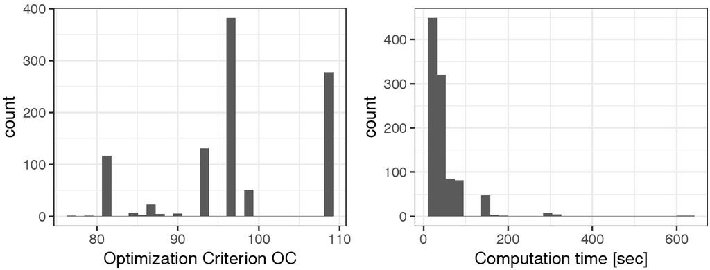
Fig. 10
The histograms of the reached optimization criterion and the execution time of EHC for HGFCBF – in-sample
OC - optimization criterion calculated as 100 * (%ARC * %ARC) / (%ASD * %MDD). The optimization criterion has been calculated from the sample of 1000 independent algorithm executions. The strategies have been working on the daily frequency, investing 20% of capital in position on each asset with rebalancing every 5 trading days. Trading from the beginning of 1998 to the end of 2013 has been simulated, with the assumption of fee equal to 0.25% of the position value.
Tab. 7
The summary of the reached optimization criterion and the execution time of the methods for HGFCBF – in-sample
| ES | EHC | GM | DEM | |||||
|---|---|---|---|---|---|---|---|---|
| OC | Time [sec] | OC | Time [sec] | OC | Time [sec] | OC | Time [sec] | |
| Minimum | 109.11 | 42193.57 | 77.29 | 12.29 | 97.04 | 113.75 | 97.04 | 9,76 |
| 1st Quantile | 109.11 | 42193.57 | 93.62 | 14.73 | 97.04 | 113.75 | 97.04 | 19.92 |
| Median | 109.11 | 42193.57 | 97.04 | 33.09 | 97.04 | 113.75 | 97.04 | 23.08 |
| Mean | 109.11 | 42193.57 | 97.82 | 42.69 | 97.04 | 113.75 | 99.01 | 27.34 |
| 2nd Quantile | 109.11 | 42193.57 | 109.11 | 36.85 | 97.04 | 113.75 | 97.04 | 29.15 |
| Max | 109.11 | 42193.57 | 109.11 | 622.17 | 97.04 | 113.75 | 109.11 | 110.93 |
| Standard deviation | 0.00 | 0.00 | 8.59 | 51.28 | 0.00 | 0.00 | 4.46 | 12.5 |
[i] OC - optimization criterion calculated as 100 * (%ARC * %ARC) / (%ASD * %MDD). The optimization criterion has been calculated from the sample of 1000 independent algorithm executions. The strategies have been working on the daily frequency, investing 20% of capital in position on each asset with rebalancing every 5 trading days. Trading from the beginning of 1998 to the end of 2013 has been simulated, with the assumption of fee equal to 0.25% of the position value.
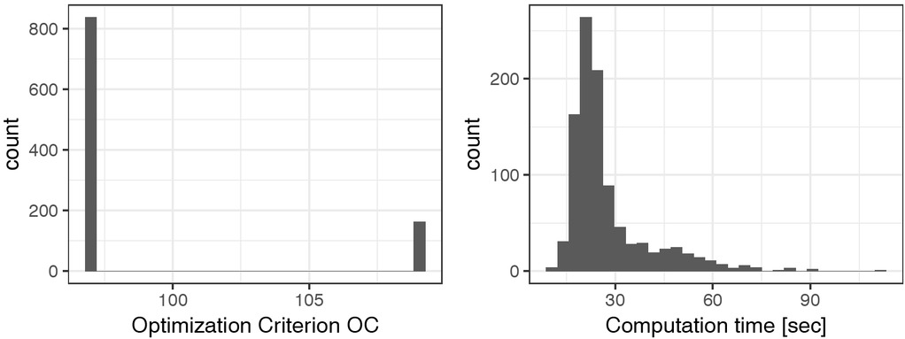
Fig. 11
The histograms of the reached optimization criterion and the execution time of DEM for HGFCBF – in-sample
OC - optimization criterion calculated as 100 * (%ARC * %ARC) / (%ASD * %MDD). The optimization criterion has been calculated from the sample of 1000 independent algorithm executions. The strategies have been working on the daily frequency, investing 20% of capital in position on each asset with rebalancing every 5 trading days. Trading from the beginning of 1998 to the end of 2013 has been simulated, with the assumption of fee equal to 0.25% of the position value.
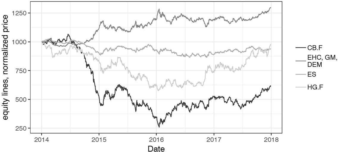
Fig. 12
The equity lines of the strategies selected by the different methods for HGFCBF – out-of-sample
SPX - S&P500 Index, DAX - Deutscher Aktienindex, ES, EHC, GD, DEM - equity line of the median strategy resulted from respectively Exhaustive Search, Extended Hill Climbing, Grid Method and Differential Evolution Method. Prices of the both assets have been normalized in order to have initial value equal to 1000. The equity line has been calculated for the strategy working on daily frequency, investing 20% of capital in position on each asset with rebalancing every 5 trading days. Trading from the beginning of 2014 to the end of 2017 has been simulated, with the assumption of fee equal to 0.25% of the position value.
Tab. 8
Mean and median optimization criterion reached by the different methods, referred to the ES method in percent – in-sample
| ES | Grid | EHC median | DEM median | EHC mean | DEM mean | |
|---|---|---|---|---|---|---|
| SPXDAX | 100 | 99.19 | 99.19 | 99.19 | 97.62 | 99.42 |
| AAPLMSFT | 100 | 100.00 | 100.00 | 100.00 | 99.55 | 99.92 |
| HGFCBF | 100 | 88.94 | 88.94 | 88.94 | 89.65 | 90.74 |
[i] SPXDAX - case of trading on S&P500 Index and Deutscher Aktienindex, AAPLMSFT - case of trading on Apple Inc. and Microsoft Corp. stocks, HGFCBF - case of trading on High-Grade Copper and Crude Oil futures. ES - the Exhaustive Search, EHC - the Extended Hill Climbing, DEM - the Differential Evolution. The simulations has been performed for the strategy working on daily frequency, investing 20% of capital in position on each asset with rebalancing every 5 trading days. Trading from the beginning of 1998 to the end of 2013 has been simulated, with the assumption of fee equal to 0.25% of the position value.
Tab. 9
Mean and median computation time of the methods, referred to the ES method in percent
| ES | Grid | EHC median | DEM median | EHC mean | DEM mean | |
|---|---|---|---|---|---|---|
| SPXDAX | 100 | 0.35 | 0.08 | 0.09 | 0.12 | 0.12 |
| AAPLMSFT | 100 | 0.46 | 0.06 | 0.07 | 0.08 | 0.07 |
| HGFCBF | 100 | 0.27 | 0.08 | 0.05 | 0.10 | 0.06 |
[i] SPXDAX - case of trading on S&P500 Index and Deutscher Aktienindex, AAPLMSFT - case of trading on Apple Inc. and Microsoft Corp. stocks, HGFCBF - case of trading on High-Grade Copper and Crude Oil futures. ES - the Exhaustive Search, EHC - the Extended Hill Climbing, DEM - the Differential Evolution. The simulations has been performed for the strategy working on daily frequency, investing 20% of capital in position on each asset with rebalancing every 5 trading days. Trading from the beginning of 1998 to the end of 2013 has been simulated, with the assumption of fee equal to 0.25% of the position value.
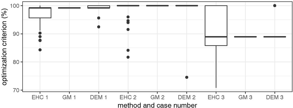
Fig. 13
The boxplot of the optimization criterion of strategies selected by the machine learning methods, as a percentage of the global maxima found by the Exhaustive Search
The samples were denoted by the algorithm acronym and the number of trading case, so 1, 2 and 3 stands for respectively SPXDAX, AAPLMSFT and HGFCBF. The box plots present the empirical distribution quartiles and highlight the outliers. Half of the observations are inside the corresponding box, when the line inside marks the median. The observation was considered as an outlier and marked by a circle if the distance from both first and third quartile (from the nearest side of the box) was higher than 1.5 interquartile range. The range of observations, without outliers was marked by the whiskers. That type of box plot was often called the Turkey Box Plot. It was worth to notice that the box plots of the Grid Method results were just a line because the results of that method were deterministic.
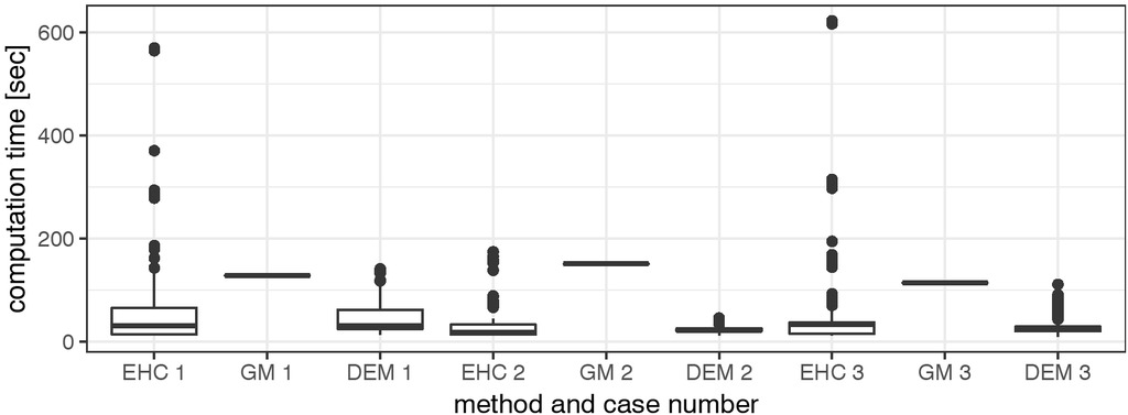
Fig. 14
The boxplot of machine learnings methods’ computation time empirical distribution
The samples were denoted by the algorithm acronym and the number of trading case, so 1, 2 and 3 stands for respectively SPXDAX, AAPLMSFT and HGFCBF. The box plots presents the empirical distribution quartiles and highlight the outliers. A half of the observations are inside the corresponding box, when the line inside marks the median. The observation was considered as an outlier and marked by a circle if the distance from both first and third quartile (from the nearest side of the box) was higher than 1.5 interquartile range. The range of observations, without the outliers was marked by the whiskers. That type of box plot was often called the Turkey Box Plot. It was worth to notice that the box plots of Grid Method results were just a line because the results of that method were deterministic.