
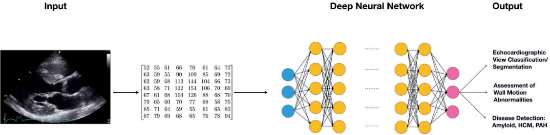
Figure 1.
Schematic of a deep neural network for imaging data. The input data often is down-sampled to a fixed height and width and nonimaging related data removed to prevent information about the target label from entering the training data. The input image data is represented to the algorithm as a fixed-size matrix corresponding to the image's pixel intensities in standard color channels (ie, red, green, blue). Each matrix (or set of matrices for a color image) represents an image that is fed into the first layer of the neural network (blue nodes). Subsequent layers of the neural network (yellow nodes) can be customized to perform a wide range of functions to the input matrix, transforming the data in a highly flexible way before feeding the data to the next layer of nodes. Deeper layers of nodes tend to learn complex interactions and higher level “features” derived from the input matrix. Each node in each layer of the network adjusts its weights during training, and the entire network is trained using the provided output labels in the training data. Different neural network architectures can be used to achieve object detection, disease classification or segmentation. HCM: hypertrophic cardiomyopathy; PAH: pulmonary arterial hypertension
Table 1.
| TYPE OF MACHINE LEARNING (ML) | DESCRIPTION | COMPUTATIONAL TECHNIQUES | EXAMPLES IN CARDIOVASCULAR IMAGING AND DATA SOURCES |
|---|---|---|---|
| Supervised learning | The data is labeled for the outcome of interest. The ML algorithm learns what features from the data drive prediction of the outcome. | Regression analysis, support vector machines, tree-based methods, neural networks (deep learning) | Madani et al. (echocardiographic data, deep learning)6 Zhang et al. (echocardiographic data, deep learning)7 Tabassian et al. (rest and stress echocardiographic data)8 Narula et al. (echocardiographic data)9 Sengupta et al. (speckle tracking echocardiographic data)10 Kusunose et al. (echocardiographic data, deep learning)11 Samad et al. (echocardiographic data)14 Kang et al. (cardiac computed tomography)15 Motwani et al. (cardiac computed tomography)16 Haro Alonso et al. (myocardial perfusion data)17 |
| Unsupervised learning | Key relationships and similarities are identified in a dataset without prior labels or annotations. | Principal component analysis, cluster analysis | Shah et al. (echocardiographic data)12 Lancaster et al. (echocardiographic data)13 |
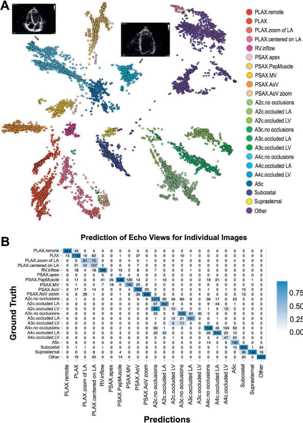
Figure 2.
Successful discrimination of echocardiographic views using convolutional neural networks. (A) Each cluster of test images corresponds to one of 23 different echocardiographic views, including apical views with or without occlusion of the left atrium. Echocardiographic still images provide examples of a 4-chamber view with and without occlusion of the left atrium. (B) Successful and unsuccessful view classifications within a matrix representation of the test data set. Successful classifications are shown as numbers along the diagonal, whereas misclassifications are indicated as off-diagonal entries. A2c: apical 2-chamber; A3c: apical 3-chamber; A4c: apical 4-chamber; echo: echocardiogram; LV: left ventricular; PLAX: parasternal long axis. Image reproduced from Zhang et al. (Open Access).7
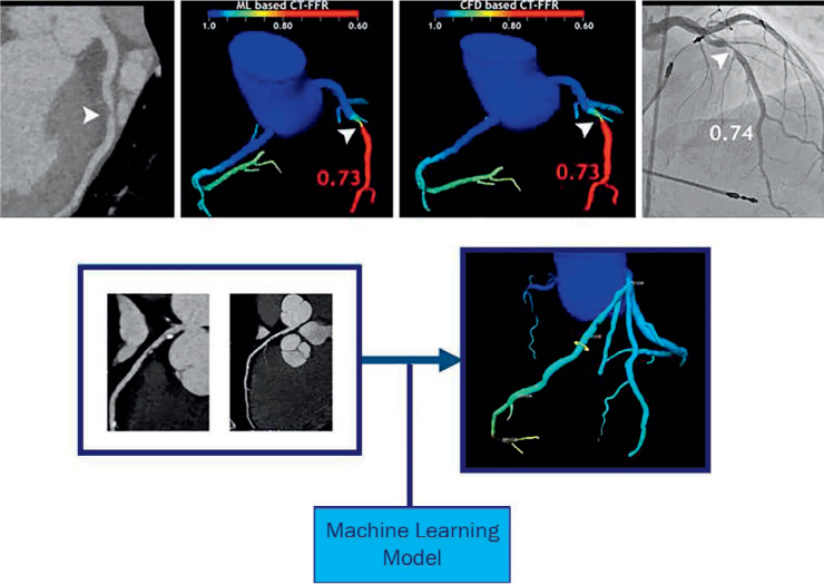
Figure 3.
Coronary stenosis (arrowheads) are displayed in different imaging methods. (a) Coronary computed tomography (CT). (b) Calculation of fractional flow reserve (FFR) with a machine learning (ML) algorithm. (c) FFR calculated with computational fluid dynamics. (d) Measurement of the stenosis during invasive coronary angiography. (e) From coronary CT to an AI-based 3-dimensional algorithm of the coronary tree displaying the FFR at different locations along the coronary arteries. Image reproduced from Siegersma et al. (Open Access).33 AI: artificial intelligence