
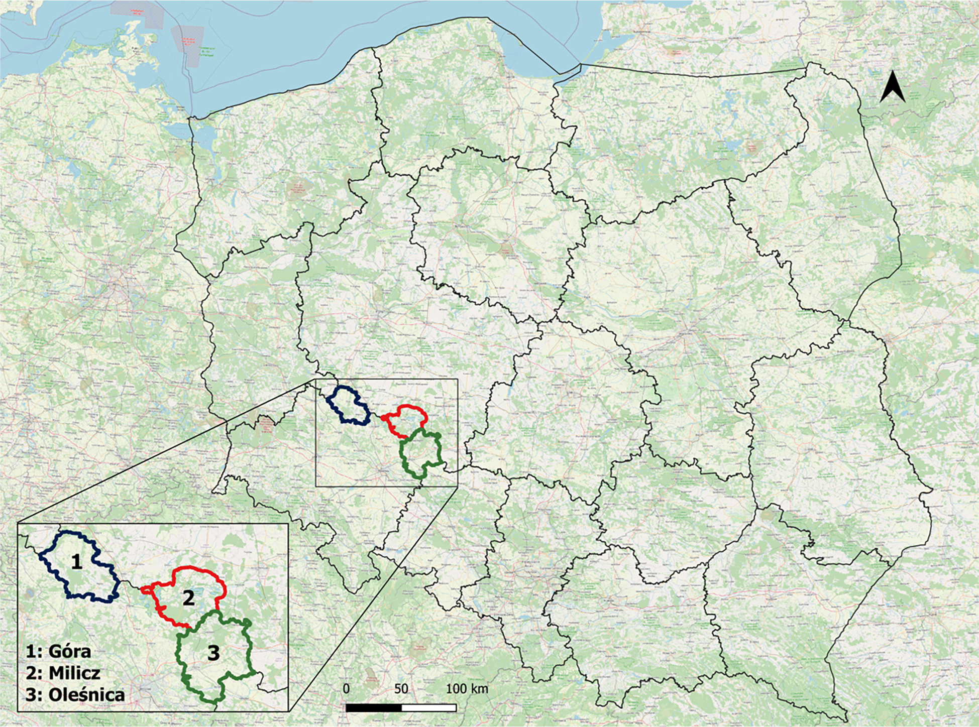
Fig. 1.
Spatial location of the research area.
Table 1.
Distribution of the basic variables.
| Variable | Category | Size | Share | ||
|---|---|---|---|---|---|
| Gender | Woman | 349 | 55% | ||
| Man | 286 | 45% | |||
| Household location | Commune centre | 338 | 53% | ||
| Up to 5 km from commune centre | 117 | 18% | |||
| More than 5 km from commune centre | 180 | 23% | |||
| County | Góra | 52 | 8% | ||
| Oleśnica | 406 | 64% | |||
| Milicz | 135 | 21% | |||
| Other | 42 | 7% | |||
| Household economic condition | Bad | 45 | 7% | ||
| Moderate | 114 | 18% | |||
| Good | 476 | 75% | |||
| Level of car utilisation | No utilisation | 123 | 19% | ||
| Some destinations | 406 | 64% | |||
| All destinations | 106 | 17% | |||
| Scale | Min | Max | M | SD | |
|---|---|---|---|---|---|
| Level of activity (number of activities) – Sum | Low – High | 0 | 12 | 6.58 | 2.43 |
| Assessment of PT frequency – Mean | Bad – Good | 1 | 5 | 2.20 | 0.88 |
| Attitude towards public transport – Mean | Positive – Negative | 1.50 | 5 | 3.22 | 0.59 |
Table 2.
Level of activity vs. level of car utilisation.
| No utilisation of private car | Utilisation of private car – some destinations | Utilisation of private car – all destinations | In total | |||||
|---|---|---|---|---|---|---|---|---|
| N | % | N | % | N | % | N | % | |
| Low level of activity | 26 | 21.10% | 94 | 23.20% | 7 | 6.60% | 127 | 20.00% |
| Moderate level of activity | 77 | 62.60% | 238 | 58.60% | 73 | 68.90% | 388 | 61.10% |
| High level of activity | 20 | 16.30% | 74 | 18.20% | 26 | 24.50% | 120 | 18.90% |
| In total | 123 | 100.00% | 406 | 100.00% | 106 | 100.00% | 635 | 100.00% |
Table 3.
Ordinal regression coefficients for the level of respondents’ activity (Model I) and the level of car utilisation (Model II) (higher coefficient = higher level of activity or car utilisation).
| Coefficients | ||
|---|---|---|
| Model I | Model II | |
| Gender = woman | 0.369* | –0.121 |
| Gender = man | ref. | ref. |
| Economic condition = bad | –1.052*** | –0.254 |
| Economic condition = moderate | 0.115 | –0.578* |
| Economic condition = good | ref. | ref. |
| HH location = more than 5 km from commune centre | –0.540** | 0.717** |
| HH location = up to 5 km from commune centre | 0.107 | 1.026*** |
| HH location = commune centre | ref. | ref. |
| County = other counties | –0.380 | –1.016 |
| County = Oleśnica | 0.233 | –0.98 |
| County = Milicz | 0.568 | –0.512 |
| County = Góra | ref. | ref. |
| Car utilisation = no | –0.775** | – |
| Car utilisation = some destinations | –0.784*** | – |
| Car utilisation = all destinations | ref. | – |
| Frequency of PT = bad assessment | – | 0.686** |
| Frequency of PT = moderate assessment | – | –0.114 |
| Frequency of PT = good assessment | – | ref. |
| Attitudes towards public transport = positive | – | –0.465* |
| Attitudes towards public transport = neutral | – | 0.149 |
| Attitudes towards public transport = negative | – | ref. |
| Model fitting (χ2) | 48.081*** | 80.697*** |
| Goodness of fit (Pearson χ2) | 232.438 | 421.882 |
| Goodness of fit (Deviance χ2) | 262.101 | 387.406 |
| Pseudo-R2 Nagelkerke | 0.09 | 0.16 |
| Test of parallel lines (χ2) | 16.116 | 17.436 |
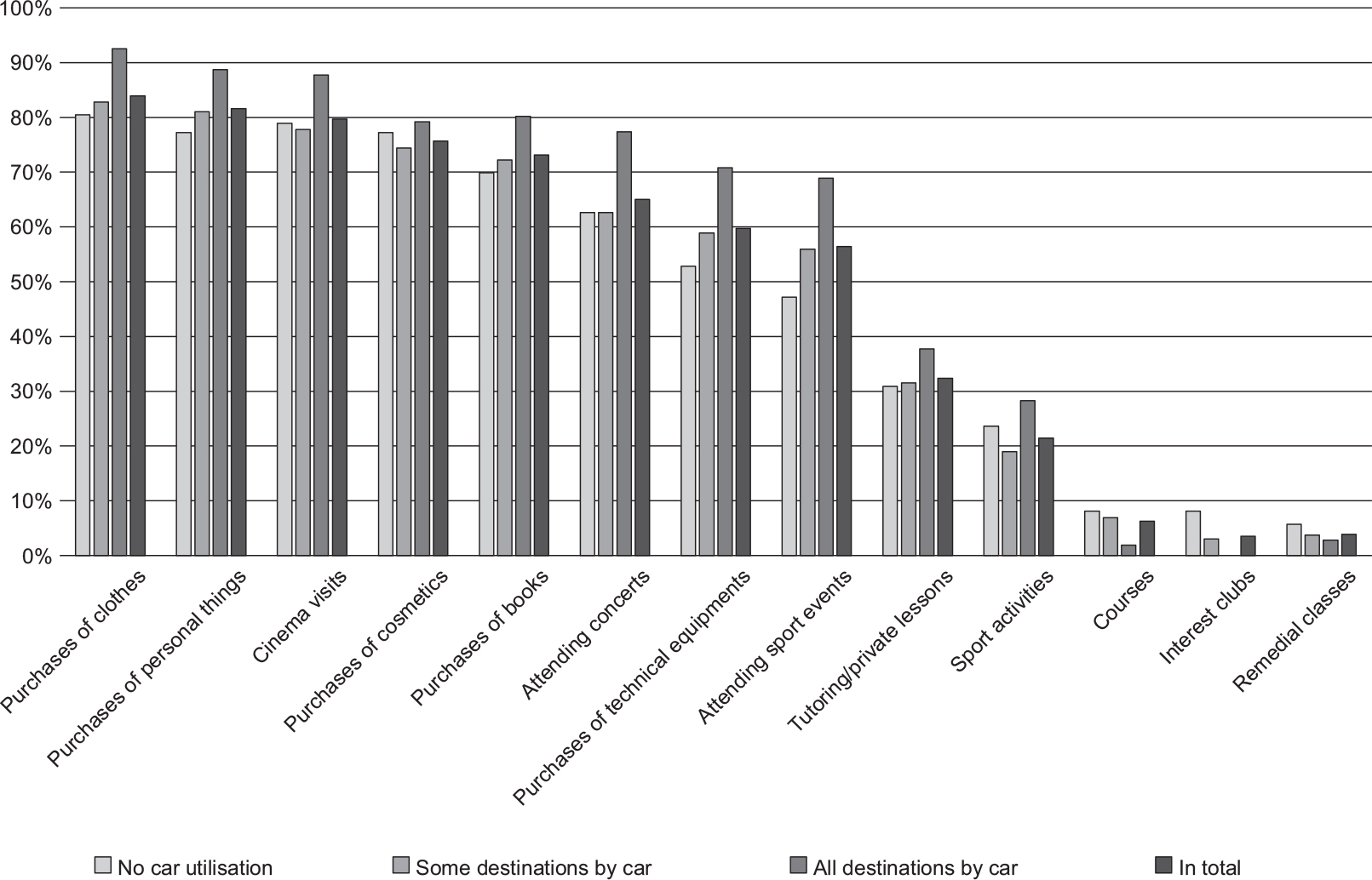
Fig. 2.
(Independent) performance of particular activities by respondents with different levels of car use (independently) doing certain activities.
Table 4.
Results of χ2 tests measuring differences in performance of particular activities by respondents with different levels of car use.
| Name of activity | χ2 | p-value |
|---|---|---|
| Purchases of clothes | 7.193 | p=.027 |
| Purchases of personal things | 5.171 | p=.075 |
| Cinema visits | 5.148 | p=.076 |
| Purchases of cosmetics | 1.263 | p=.532 |
| Purchases of books | 3.513 | p=.173 |
| Attending concerts | 8.479 | p=.014 |
| Purchases of technical equipments | 7.89 | p=.019 |
| Attending sport events | 10.997 | p=.004 |
| Tutoring/private lessons | 1.642 | p=.440 |
| Sport activities | 4.769 | p=.092 |
| Courses | 4.433 | p=.109 |
| Interest clubs | 12.105 | p=.002 |
| Remedial classes | 1.405 | p=.495 |
Table 5.
Results of χ2 tests measuring differences in performance of particular activities by respondents from peripheral locations.
| Name of activity | χ2 | p-value |
|---|---|---|
| Purchases of clothes | 6.637 | p=.036 |
| Purchases of personal things | 3.105 | p=.212 |
| Cinema visits | 9.329 | p=.009 |
| Purchases of cosmetics | 6.218 | p=.045 |
| Purchases of books | 5.263 | p=.072 |
| Attending concerts | 12.740 | p=.002 |
| Purchases of technical equipments | 3.279 | p=.194 |
| Attending sport events | 9.219 | p=.010 |
| Tutoring/private lessons | 5.412 | p=.067 |
| Sport activities | 10.134 | p=.006 |
| Courses | 4.567 | p=.102 |
| Interest clubs | 5.207 | p=.074 |
| Remedial classes | 0.792 | p=.673 |
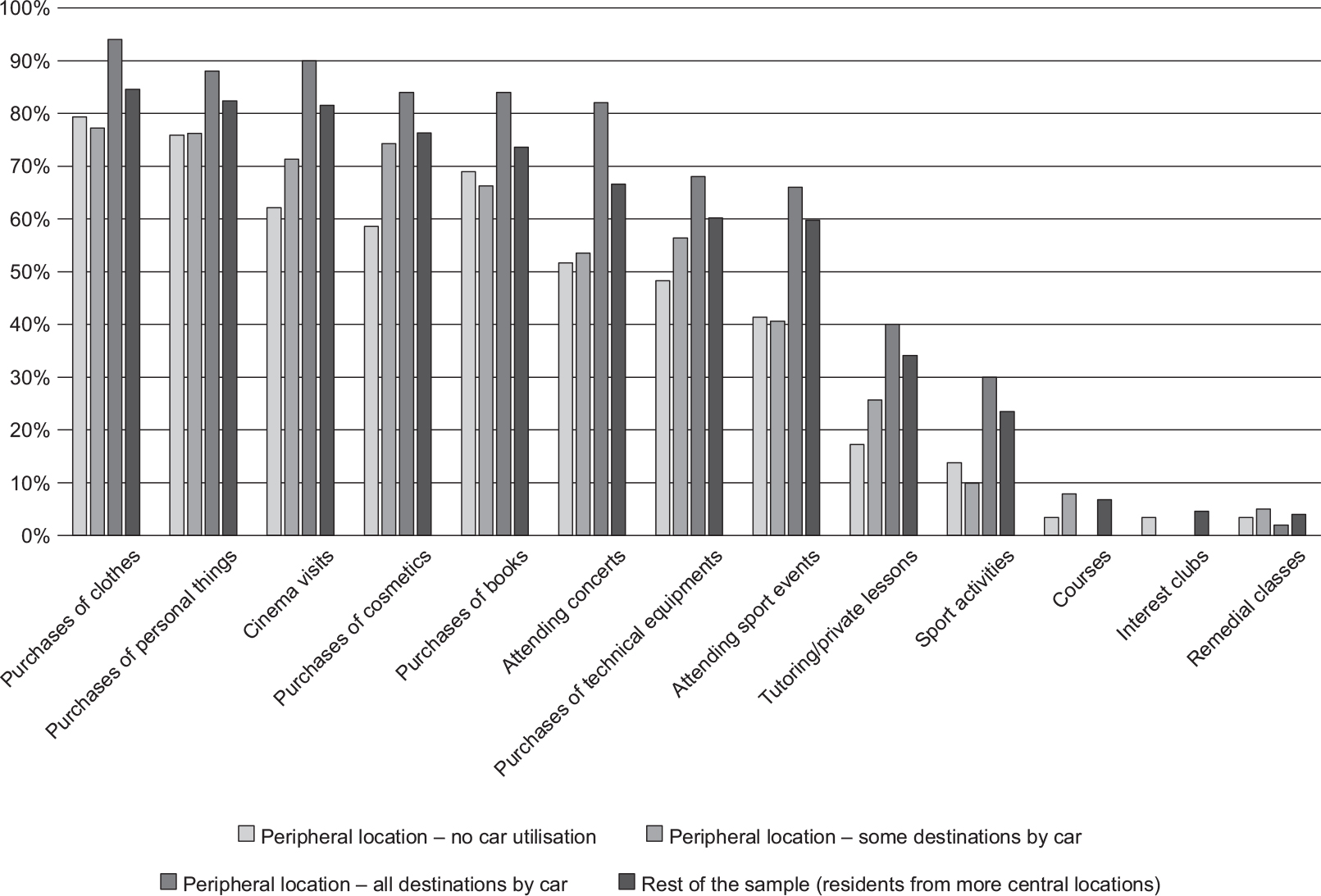
Fig. 3.
(Independent) performance of particular activities by respondents from peripheral locations (more than 5 km from the centre of the commune) and with different levels of car use.
Table 6.
Expected improvements in public transport in the household location.
| Expected improvement | Level of activity | Level of car utilisation | In total | ||||
|---|---|---|---|---|---|---|---|
| Low | Moderate | High | No utilisation | 1–2 destinations | All destinations | ||
| % in column* | |||||||
| Increased frequency of services | 47% | 56% | 59% | 63% | 56% | 51% | 54% |
| New public transport connections | 23% | 31% | 33% | 33% | 26% | 31% | 29% |
| Lower ticket prices | 34% | 28% | 26% | 30% | 28% | 30% | 29% |
| Improved punctuality | 15% | 18% | 13% | 27% | 19% | 12% | 16% |
| Increased comfort of journeys | 8% | 15% | 18% | 7% | 15% | 13% | 13% |
| Upgraded bus stop infrastructure | 5% | 7% | 5% | 13% | 5% | 5% | 6% |
| Increased feeling of security | 3% | 4% | 3% | 3% | 5% | 3% | 4% |
| Upgraded fleet | 3% | 2% | 0% | 3% | 1% | 3% | 2% |
| Other factors | 3% | 1% | 3% | 0% | 2% | 1% | 1% |
| Nothing | 23% | 13% | 13% | 3% | 14% | 20% | 16% |