
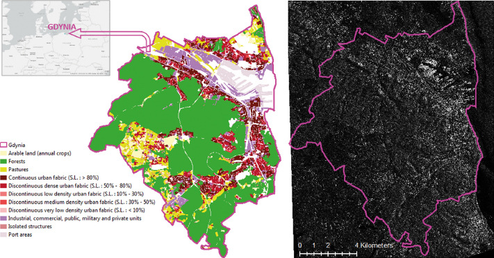
Fig. 1.
The extent of Gdynia’s boundary (purple lines) on the VV ICEYE image (right) and the visualisation of the UA database in the study area according to the UA legend (left). UA, Urban Atlas.
Table 1.
Specification of the SAR data used in the study.
| Sensor | Date | Band | Polarisation | Orbit | Mode | Spatial resolution after corrections and resampling |
|---|---|---|---|---|---|---|
| ICEYE | 19.04.2019 | X (3 cm) | VV | Ascending | SM | 2 m |
| Sentinel-1 | 27.12.2018 | C (5 cm) | VH + VV | Descending | IW | 10 m |
Table 2.
Urban Atlas classes selected for the study. These code names and colours have been used in the forth-coming presentation of results.
| Class name | Sealed Level (SL) | Codename and colour on images | Name and colour of aggregated classes |
|---|---|---|---|
| Continuous urban fabric | >80% |  CUF CUF |  Dense urban area Dense urban area |
| Discontinuous dense urban fabric | 50–80% |  DDUF DDUF | |
| Discontinuous medium density urban fabric | 30–50% |  DMDUF DMDUF | |
| Discontinuous low density urban fabric | 10–30% |  DLDUF DLDUF |  Low density urban area Low density urban area |
| Discontinuous very low density urban fabric | <10% |  DVLDUF DVLDUF | |
| Isolated structures |  IS IS | ||
| Port areas |  PA PA |  Industrial area Industrial area | |
| Industrial, commercial, public, military and private units |  ICPMAPU ICPMAPU | ||
| Arable land (annual crops) |  AL AL |  Vegetation Vegetation | |
| Forests |  F F | ||
| Pastures |  P P | ||
| UA class borders |  |
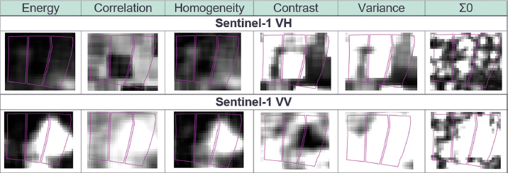
Fig. 2.
Sentinel-1 variables selected for classification. The same representative example for the Continuous urban fabric CUF class shown on orthophotomap in Fig. 5.
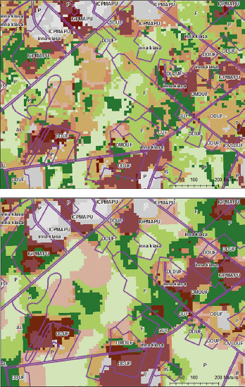
Fig. 3.
Results of supervised classification by RF (upper) and MD (lower) for Sentinel-1 with UA class outlines. The fragment shows the representation and variety of different classes in the area. The same legend is applicable as was mentioned in Table 2.
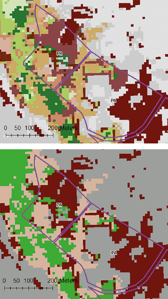
Fig. 4.
RF (100 trees) classification result on Sentinel-1 before (upper) and after aggregation to four classes (lower). Example of Port area (PA) class differentiation. The same legend is applicable as was mentioned in Table 2.
Table 3.
Sentinel-1 image classification accuracy by RF (top) and MD (bottom) algorithms – both results after aggregation.
| Class value | Vegetation | Dense urban | Low dens. urban | Industrial | Total | U_Accuracy | Kappa |
|---|---|---|---|---|---|---|---|
| RF classification | |||||||
| Vegetation | 685 | 58 | 21 | 70 | 834 | 0.821 | 0 |
| Dense urban | 29 | 140 | 5 | 162 | 336 | 0.417 | 0 |
| Low dens. urban | 196 | 66 | 17 | 98 | 377 | 0.045 | 0 |
| Industrial | 28 | 103 | 2 | 321 | 454 | 0.707 | 0 |
| Total | 938 | 367 | 45 | 651 | 2001 | 0 | 0 |
| P_Accuracy | 0.730 | 0.381 | 0.378 | 0.493 | 0 | 0.581 | 0 |
| Kappa | 0 | 0 | 0 | 0 | 0 | 0 | 0.398 |
| MD classification | |||||||
| Vegetation | 747 | 63 | 21 | 57 | 888 | 0.841 | 0 |
| Dense urban | 32 | 144 | 3 | 118 | 297 | 0.485 | 0 |
| Low dens. urban | 141 | 56 | 21 | 114 | 332 | 0.063 | 0 |
| Industrial | 18 | 104 | 0 | 362 | 484 | 0.748 | 0 |
| Total | 938 | 367 | 45 | 651 | 2001 | 0 | 0 |
| P_Accuracy | 0.796 | 0.392 | 0.467 | 0.556 | 0 | 0.637 | 0 |
| Kappa | 0 | 0 | 0 | 0 | 0 | 0 | 0.468 |
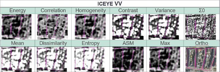
Fig. 5.
ICEYE variables selected for classification and contours of the Continuous urban fabric CUF class (as a representative example). The right-bottom orthophoto shows the scale and shape of features.
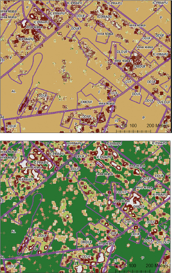
Fig. 6.
Results of classification using RF (upper) and MD (lower) on ICEYE image with UA class borders.
The same legend is applicable as was mentioned in Table 2. This representative example shows the diversity of classes.
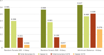
Fig. 7.
Overall classification accuracy (total and kappa) based on RF and MD classifiers for Sentinel-1 (S1, in green colours) and ICEYE (brown-orange colours).
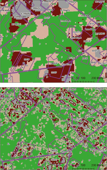
Fig. 8.
Comparison of Sentinel-1 (upper) and ICEYE (lower) results based on MD classifier, after class aggregation. The same legend is applicable as was mentioned in Table 2. This representative example shows the diversity of classes.
Table 5.
Comparison of classification results in different images and different algorithms for Continuous urban fabric class and discontinuous dense urban fabric, both in one dense urban area class; these representative examples visualise a general pattern.
| Continuous urban fabric | ||
|---|---|---|
| orthophotomap | 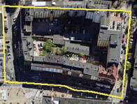 |  Dense urban area Dense urban area Low density urban area Low density urban area Industrial area Industrial area Vegetation Vegetation Urban Atlas feature Urban Atlas feature |
| Sentinel-1 | ICEYE | |
| Random Forests | 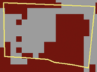 | 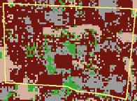 |
| Minimum Distance | 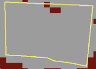 | 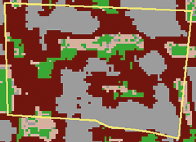 |
| Discontinuous dense urban fabric | ||
| orthophotomap | 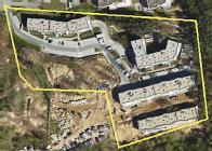 | |
| Sentinel-1 | ICEYE | |
| Random Forests | 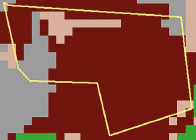 | 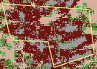 |
| Minimum Distance | 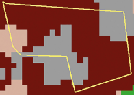 | 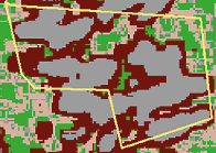 |
Table 6.
Comparison of classification results in different images and different algorithms for discontinuous low and very low density urban fabric, both in low density urban area class; these representative examples visualise a general pattern.
| Discontinuous low density urban fabric | ||
|---|---|---|
| orthophotomap | 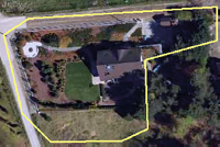 |  Dense urban area Dense urban area Low density urban area Low density urban area Industrial area Industrial area Vegetation Vegetation Urban Atlas feature Urban Atlas feature |
| Sentinel-1 | ICEYE | |
| Random Forests | 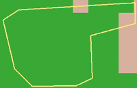 | 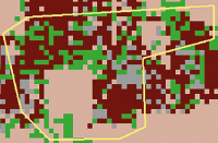 |
| Minimum Distance | 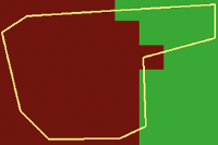 | 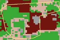 |
| Discontinuous very low density urban fabric | ||
| orthophotomap | 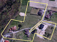 | |
| Sentinel-1 | ICEYE | |
| Random Forests | 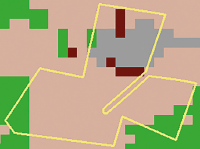 | 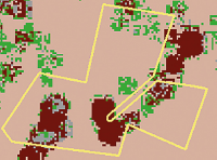 |
| Minimum Distance | 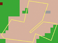 | 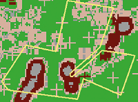 |