
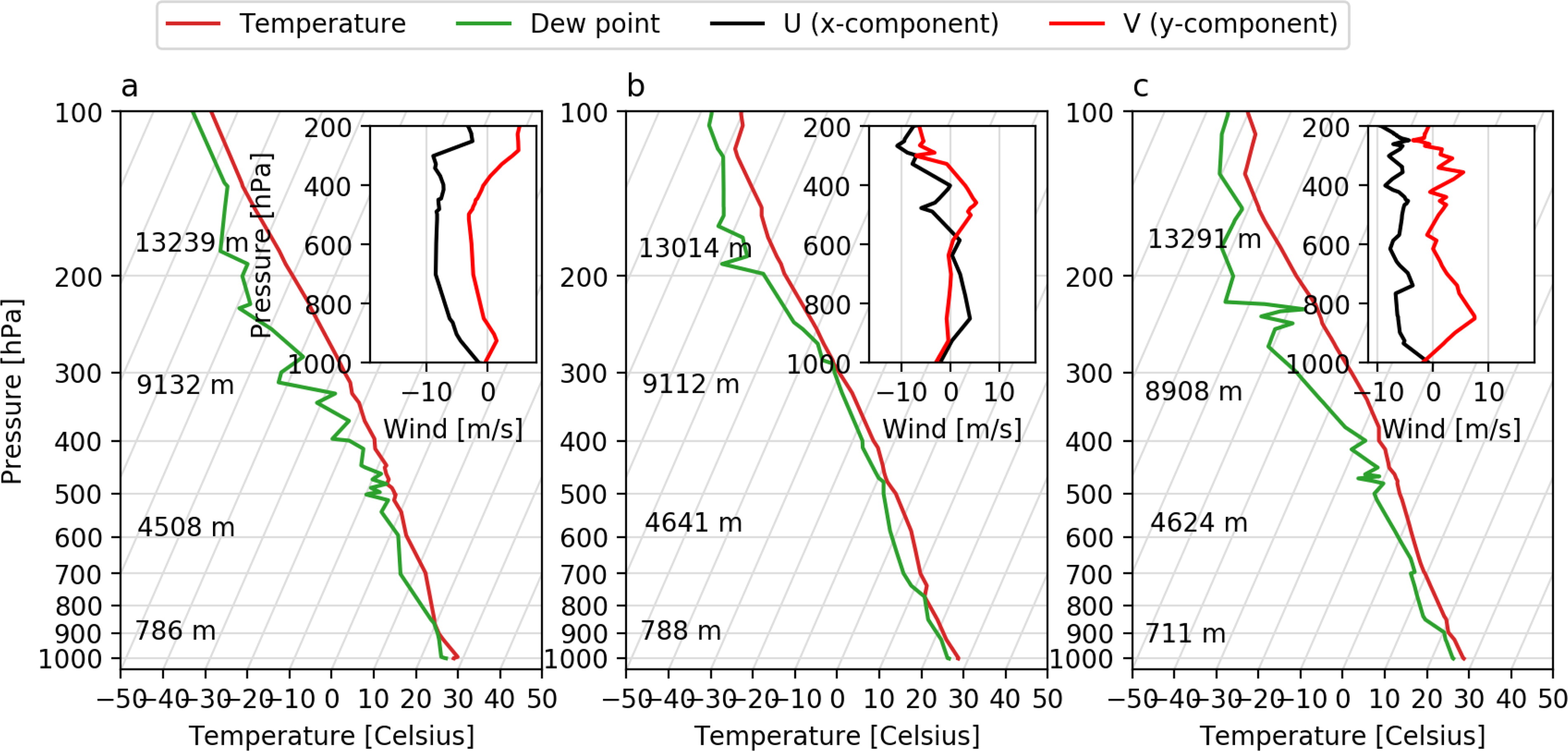
Fig. 1.
SkewT-logP and wind diagrams for the atmospheric soundings retrieved in Manaus, Brazil on April 8 (a), 2020, April 23, 2020 (b) and April 27, 2020 (c).
Table 1.
Molecular properties for the system compounds used in the simulations.
Table 2.
Different settings for the simulations.
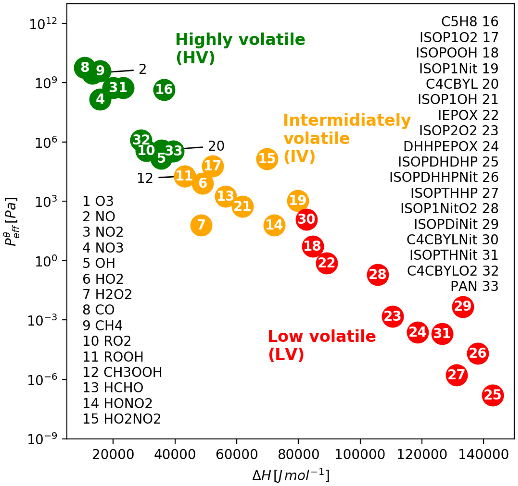
Fig. 2.
Volatility diagram for the compounds in the modelled system.
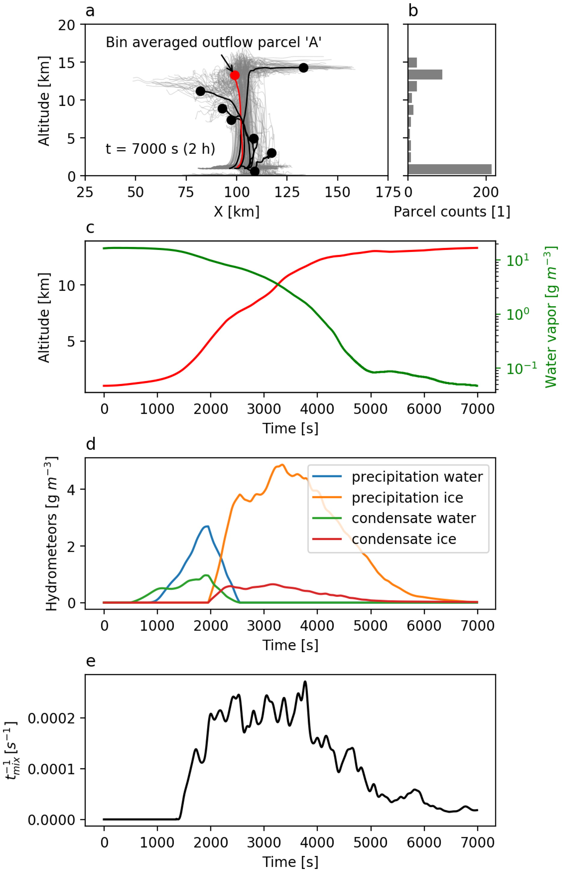
Fig. 3.
Trajectories of the 400 simulated deep convective cloud air parcels for the April 23, 2020 case (grey), parcels averaged by height bins (black), parcel A used for further analysis (red) (a), distribution of parcels according to their final altitude (b), the altitude of parcel A (red line) and the corresponding water vapour concentration (green line) (c), the total water mass of the different types of hydrometeors (d), and the reversed timescale of mixing (e).
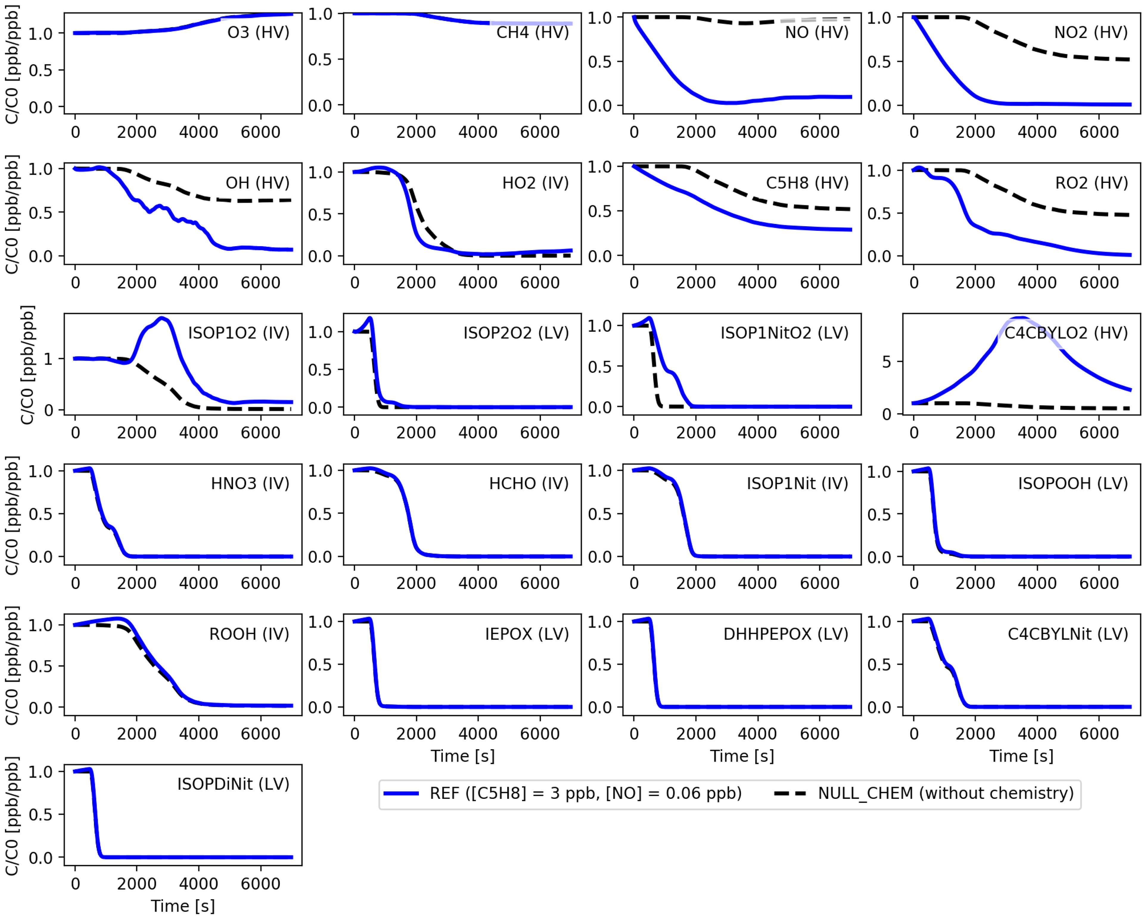
Fig. 4.
Evolution of gas phase concentrations of the 21 selected compounds (see Table 1) along the trajectory A (see Fig. 3) for the REF and NULL_CHEM simulations given in Table 2. The concentrations in ppb are normalised to the corresponding initial values also in ppb. The compound notations are followed by the corresponding volatility acronym in parentheses. Corresponding figures for all the 33 modelled species are provided in SI.
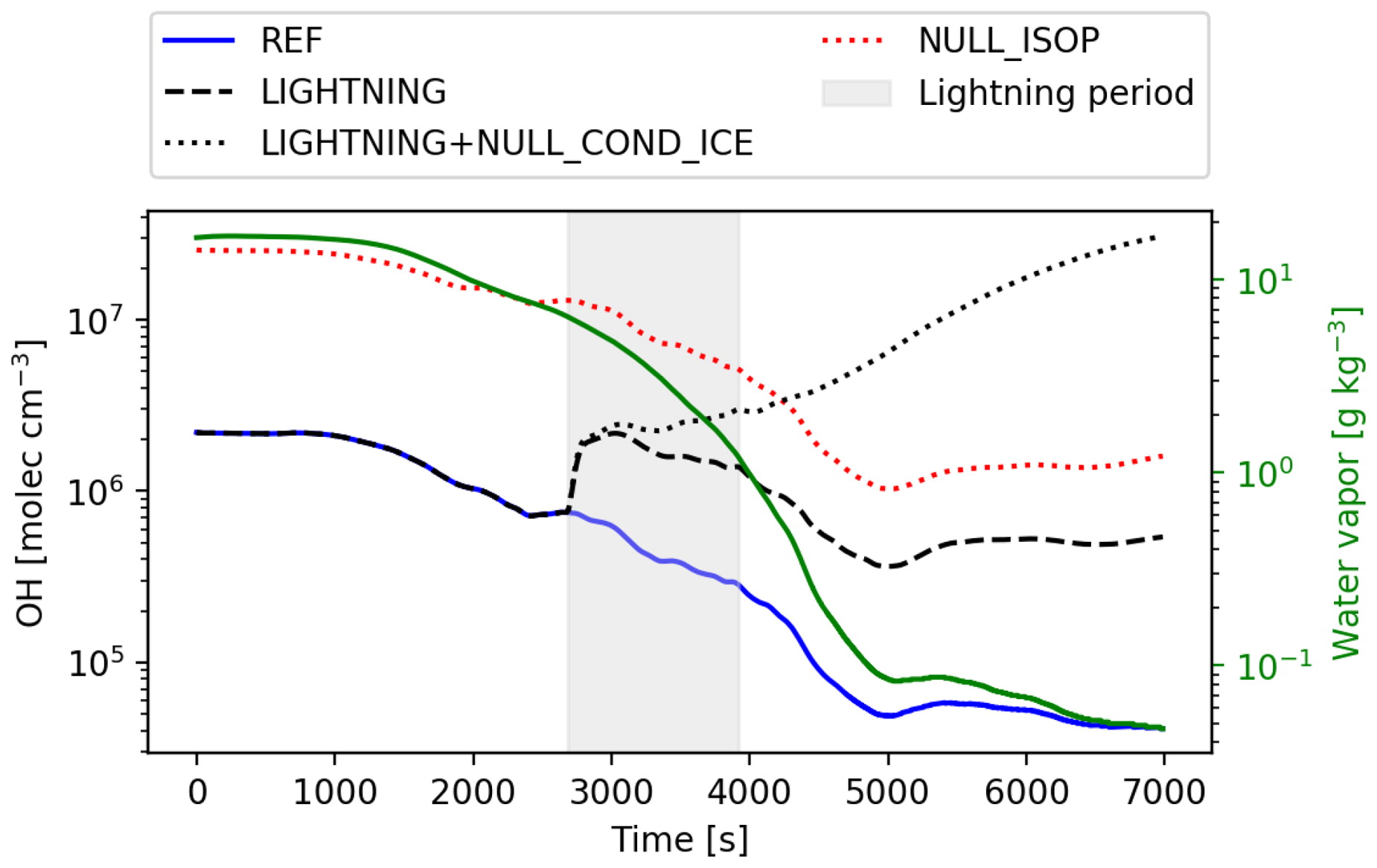
Fig. 5.
Evolution of OH along the trajectory A (see 3) for the REF (blue solid line), LIGHTNING (black dashed line), LIGHTNING + NULL_COND_ICE (black dotted line), NULL_ISOP (red dotted line) simulations as well as concentration of water vapour (or H2O, green solid line) as a function of time. Grey shaded area shows lightning period.
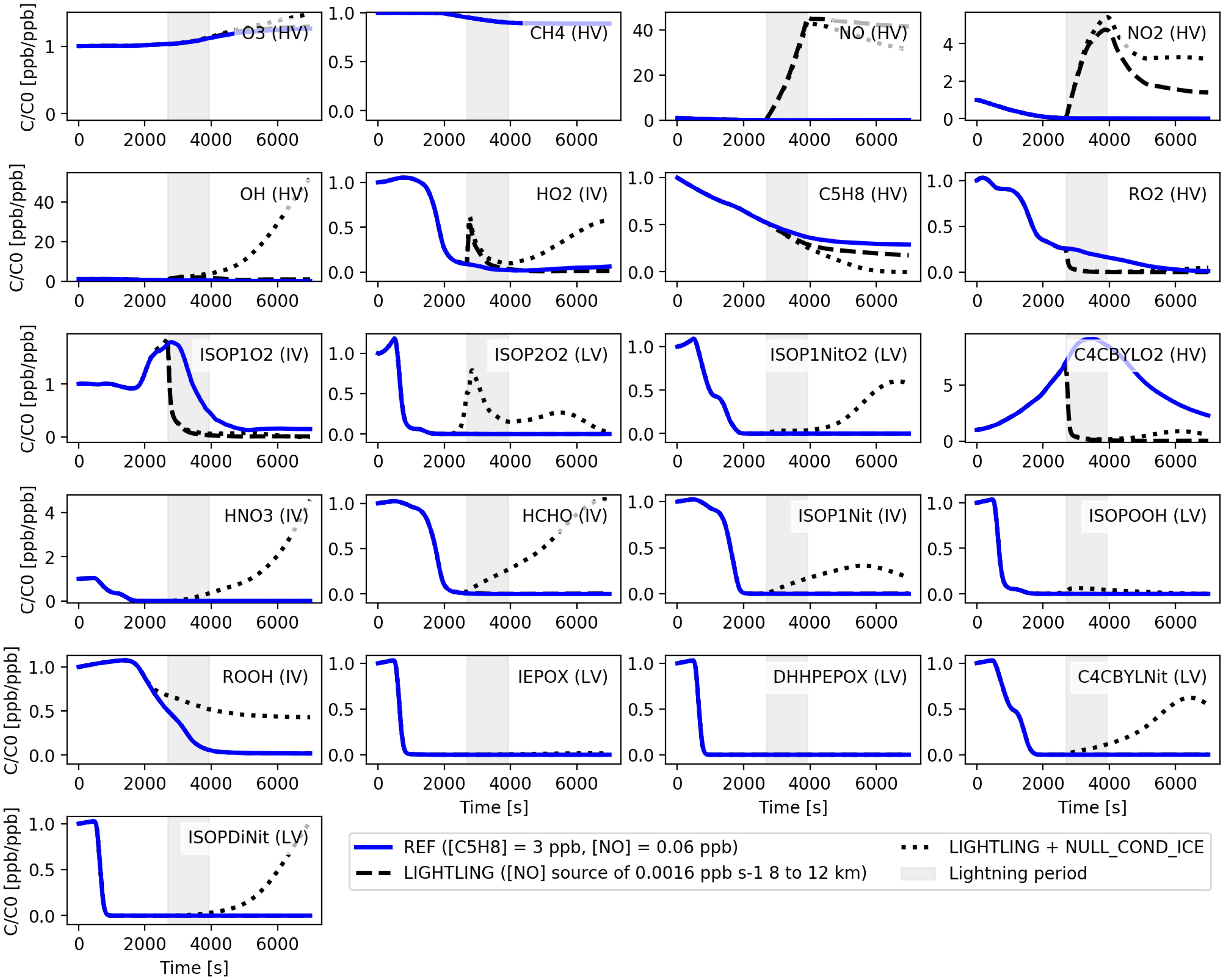
Fig. 6.
Evolution of gas phase concentrations of the 21 studied compounds (see Table 1) along the trajectory A (see Fig. 3) for the simulations REF (blue line), LIGHTNING (dashed black line) and LIGHTNING + NULL_COND_ICE (dotted black line), see Table 2. The grey shaded area denotes period of simulated lightning. The concentrations in ppb are normalised to the corresponding initial values also in ppb. The compound notations are followed by the corresponding volatility acronym in parentheses. Figures for all the 33 modelled species as well as a figure which compares the REF and LIGHTNING cases are provided in SI.
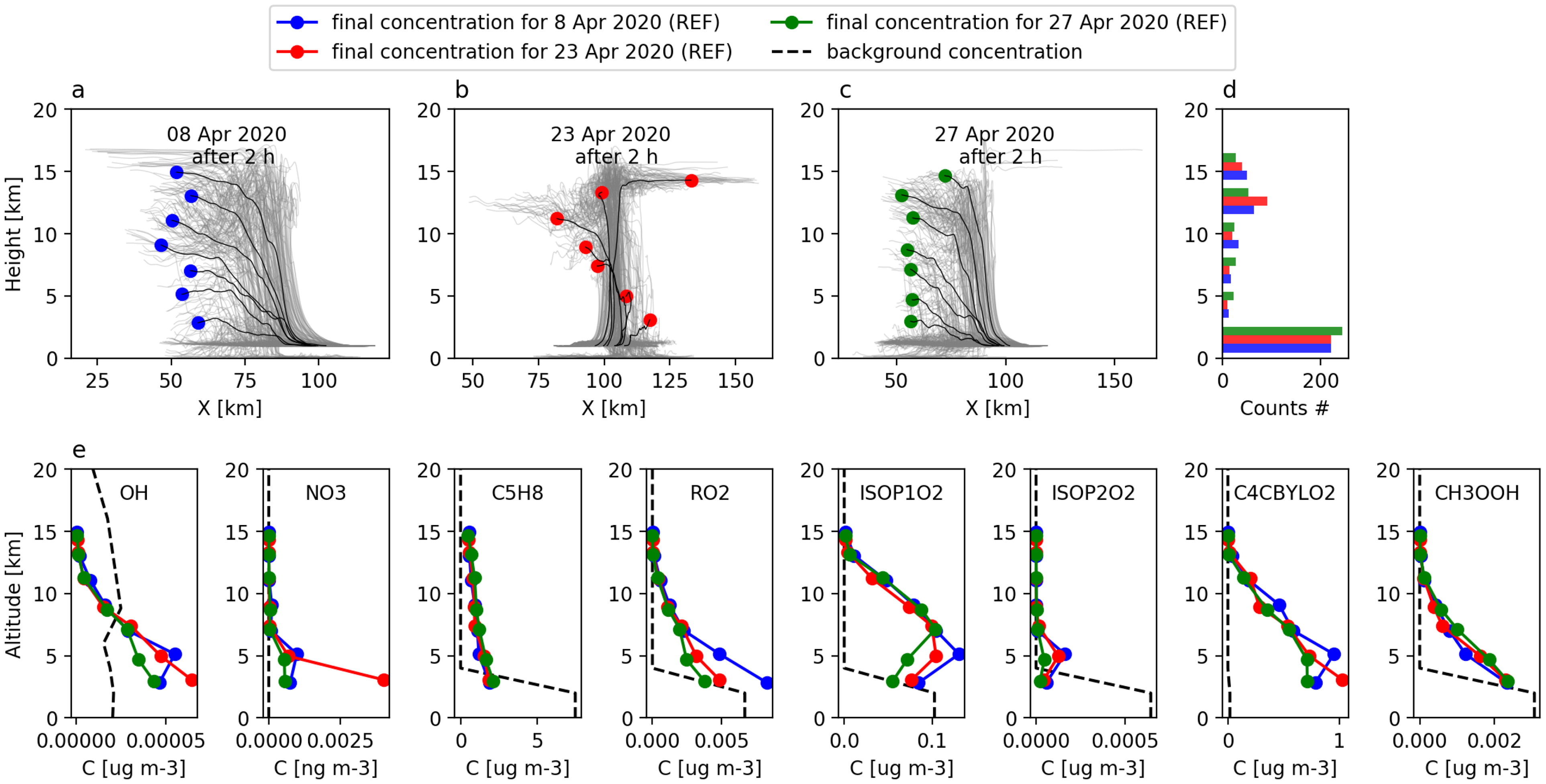
Fig. 7.
Trajectories from three different simulated deep convective cloud events (a, b and c). All parcels were divided into bins as a function of their arrival altitude and their properties were thereafter averaged (filled circles in a, b and c). Histogram of the final altitudes of the parcels (d) and chemical concentrations (e) in the out-of-cloud background (dashed line) and in the binned parcels after 2 h of simulation for three deep convective cloud cases (colored lines). Simulation settings are according to REF (see Table 2).
Table A1. Coefficients aij used for meteorological interactions.
[i] See Bardakov et al. (2020) for more details about the coefficients.
Table B1. Photolysis reactions.
[ii] b) and are the rates for reactions and with assumed values of and respectively (Tan et al., 2019).
Table B2. Chemical reactions for the system components and their rates. Part 1.