
Table 2.
Hyperparameter tuning of the GBRT model. The left-hand column names the property, and the right-hand column lists the values tested using grid search. Bold values are chosen for the final model on the basis of a 3-fold cross validation. The number of estimators is determined by early stopping as described in section 2.2, with a maximum number of estimators set to 20000.

Fig. 1.
Schematic overview of the two-step machine learning approach used in this study. Significant differences in the comparison of the simulated AOD E (blue) and the observed AOD (red) during the lockdown are interpreted as aerosol source changes.
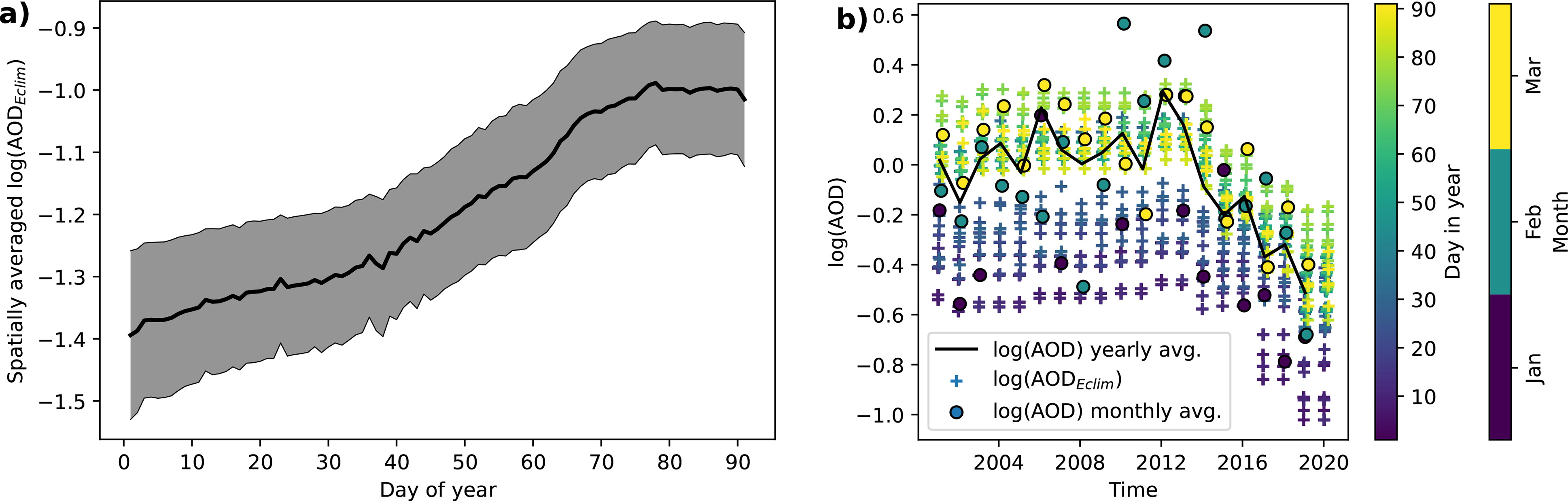
Fig. 2.
Domain-average climatologically expected log(AOD Eclim ) grouped by day of year (a)), displaying seasonal characteristics of the AOD data set. The black line represents the mean, the grey area the mean ± 1 standard deviation of the regional models. Panel b) shows an example of a log(AOD time series for Chengdu (‘+’ symbol), together with long-term variability (yearly average, black), and seasonal variability (monthly average, circles) of observed log(AOD).
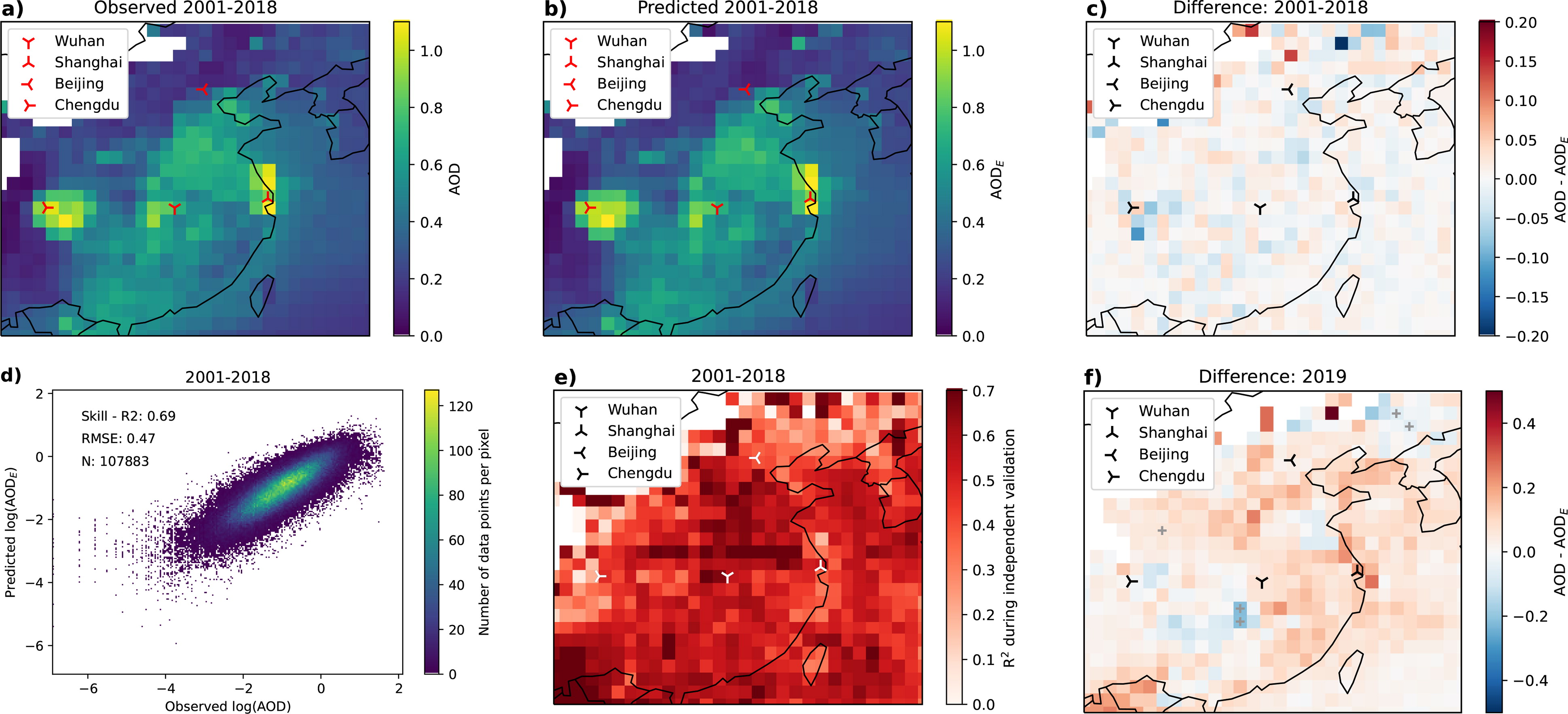
Fig. 3.
Validation of the machine-learning model predicting AOD/log(AOD) with independent test data. The top row shows average observed and predicted (backtransformed) AOD of the test data in a) and b), and their difference in c) in the study domain (20 N–45 N and 100 E–130 E). Panel d) shows a scatter plot summarizing the model skill to predict log(AOD) over the entire domain and therefore represents a combination of spatial and temporal skill. e) Spatial patterns of model skill in predicting the temporal variability of log(AOD) in each grid cell (R2). Panel f) shows the difference between observed AOD and predicted (back-transformed) AOD E , with grey ‘+’ symbols showing significance at 0.01 level of an independent two-sided t test.
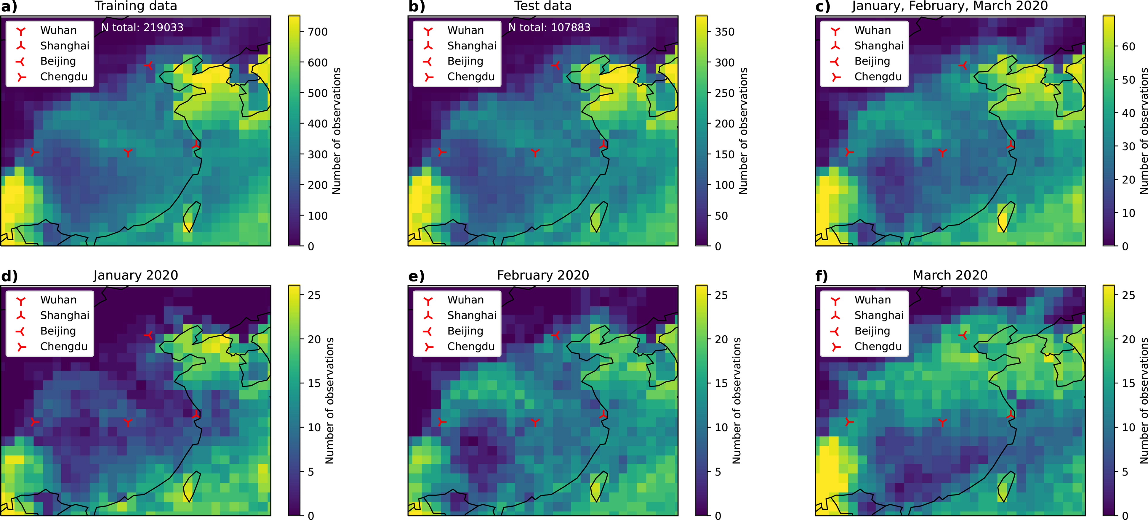
Fig. 4.
Number of valid AOD observations during a) training, b) testing, c) JFM 2020, d) January 2020, e) February 2020, and f) March 2020 in the study domain (20 N–45 N and 100 E–130 E).
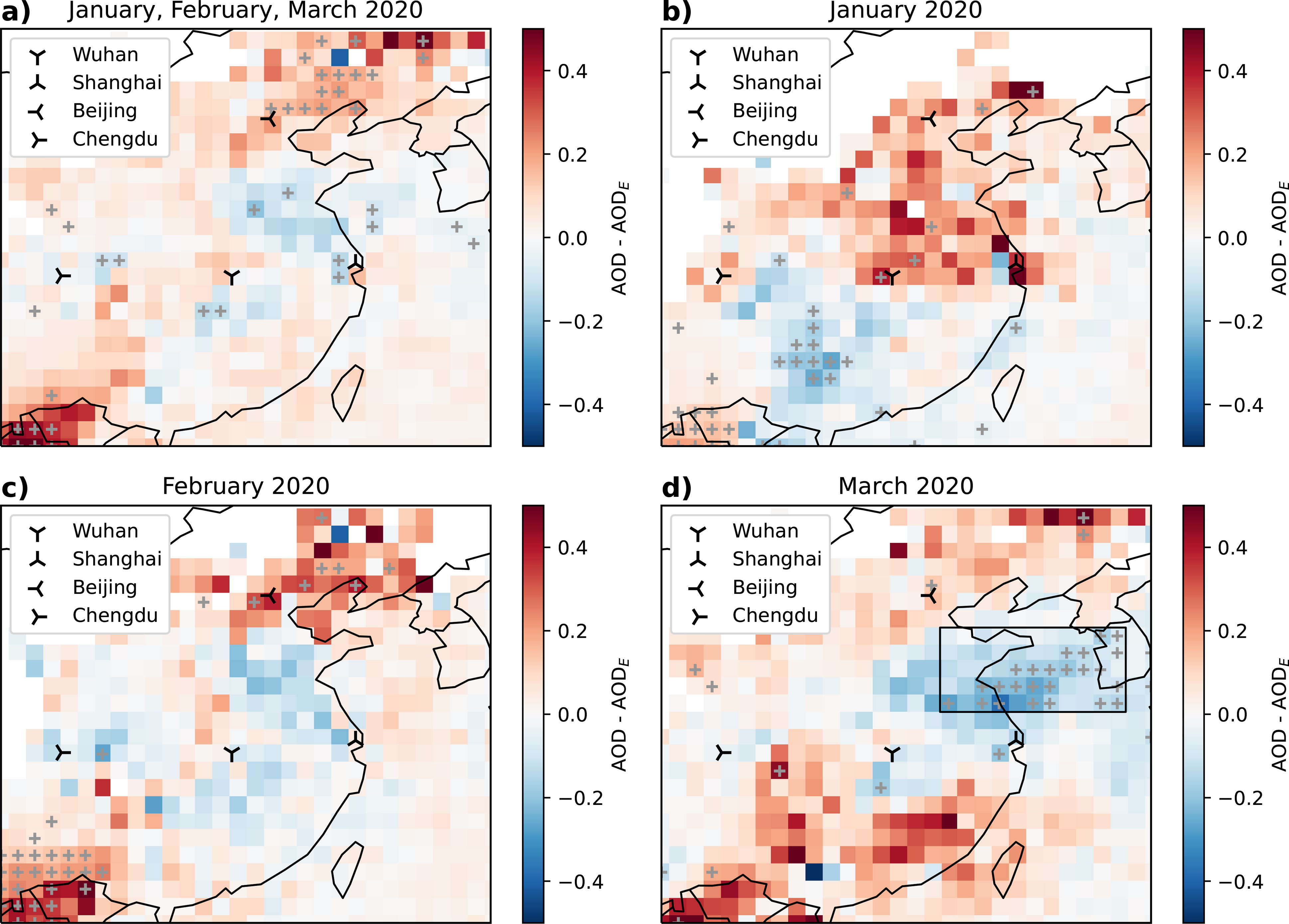
Fig. 5.
Comparison of observed AOD 2020 minus AOD E for a) JFM 2020, b) January 2020, c) February 2020, and d) March 2020 in the study domain (20 N–45 N and 100 E–130 E). Grey ‘+’ symbols show significance at 0.01 level of an independent two-sided t test. The black box in panel d) shows the region that is further investigated in Fig. 6.

Fig. 6.
Comparison of observed AOD and predicted AOD E and AOD Eclim distributions of the region shown as a box in Fig. 5d) for test data in the time period of 2001–2018 (a)), and March 2020 (b)). Predicted log(AOD E ) and log(AOD Eclim ) are back-transformed for the comparison. Thin vertical lines shows the median of the distributions.

Fig. 7.
Comparison of climatologically expected AOD Eclim minus AOD E for JFM 2020 in the study domain (20 N–45 N and 100 E–130 E), grey ‘+’ symbols show significance at 0.01 level of an independent two-sided t test.
Table 1.
Overview of the input features used to predict log(AOD). Input features in bold are those used by the final model after recursive feature elimination.