
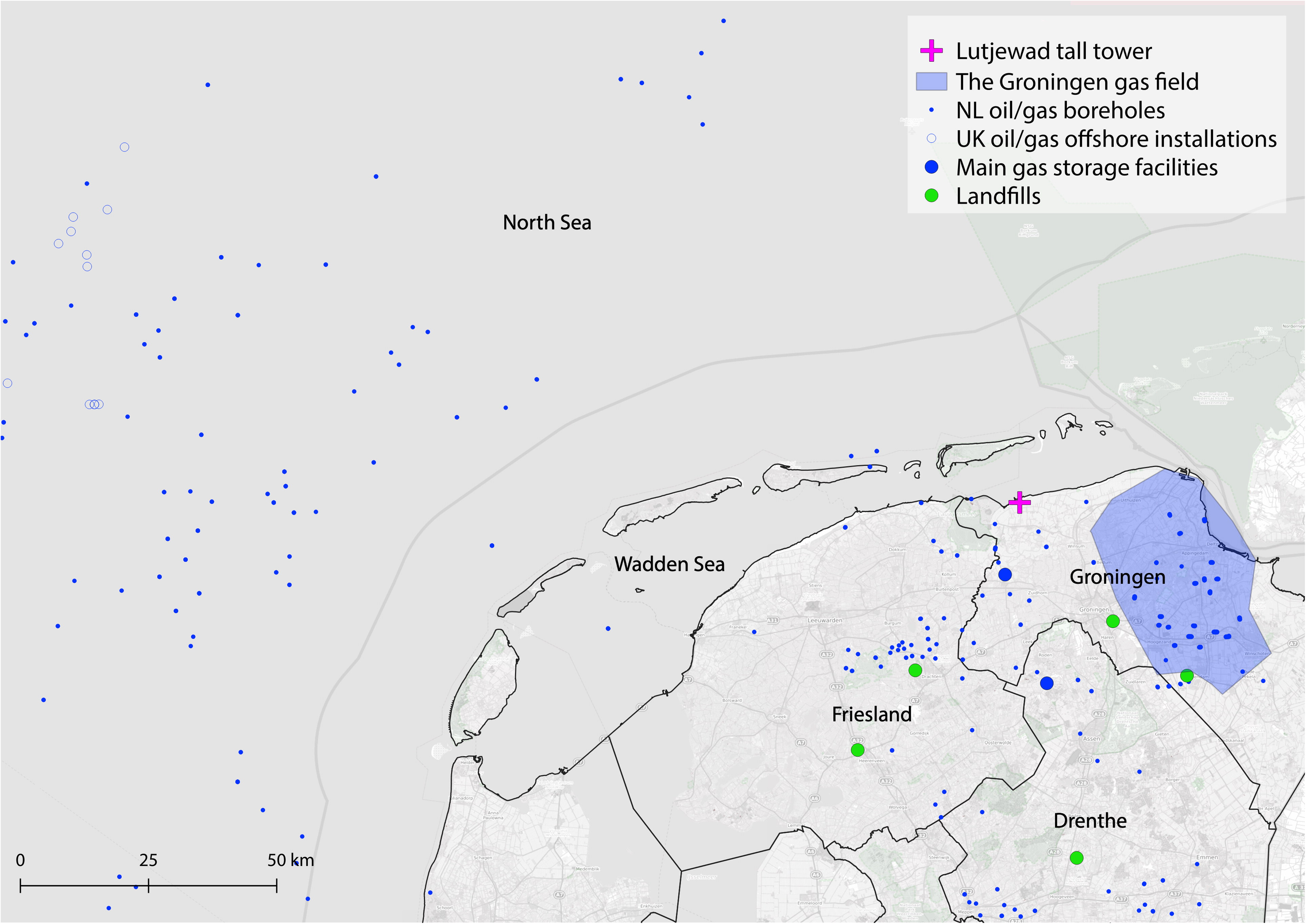
Fig. 1.
Location of the measurement site (magenta cross) and potential on-shore and off-shore methane sources. Sources: https://www.openstreetmap.org, OSPAR Commission (2015), Vlek (2018), Ministerie van Economische Zaken, TNO (2018), and Stortplaatsen in Nederland (2019).
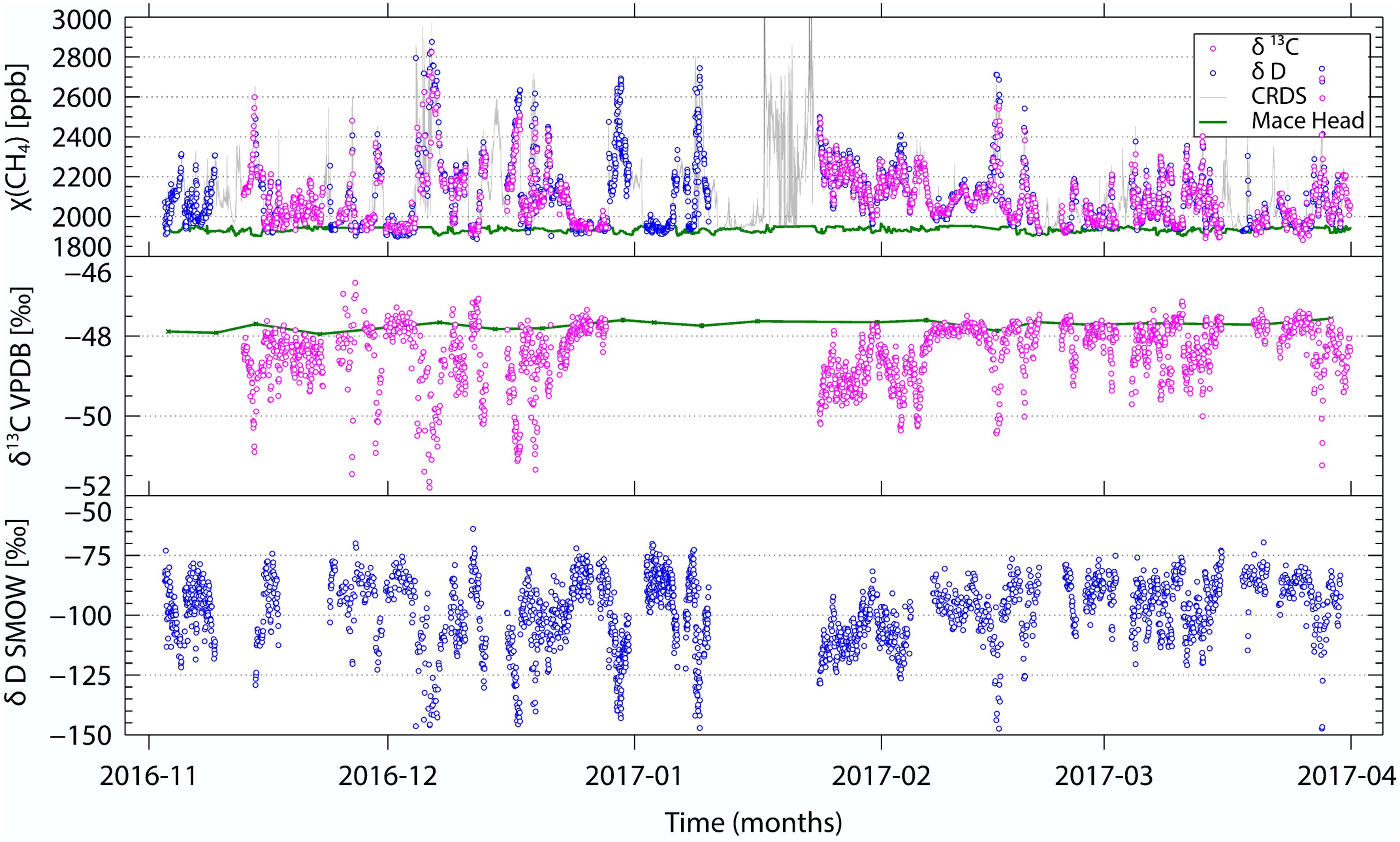
Fig. 2.
Overview of the entire dataset, including corrections made on IRMS χ(CH4) to match the CDRS records. The Mace Head δ 13C-CH4 data (Dlugockenky et al., 2019) was corrected by −0.11‰ according to the scale difference between the INSTAAR and the IMAU measurements evaluated in Umezawa et al. (2018).
Table 2.
Overall contribution from each source type to χ(CH4) from CHIMERE, in [%] ± 1σ.
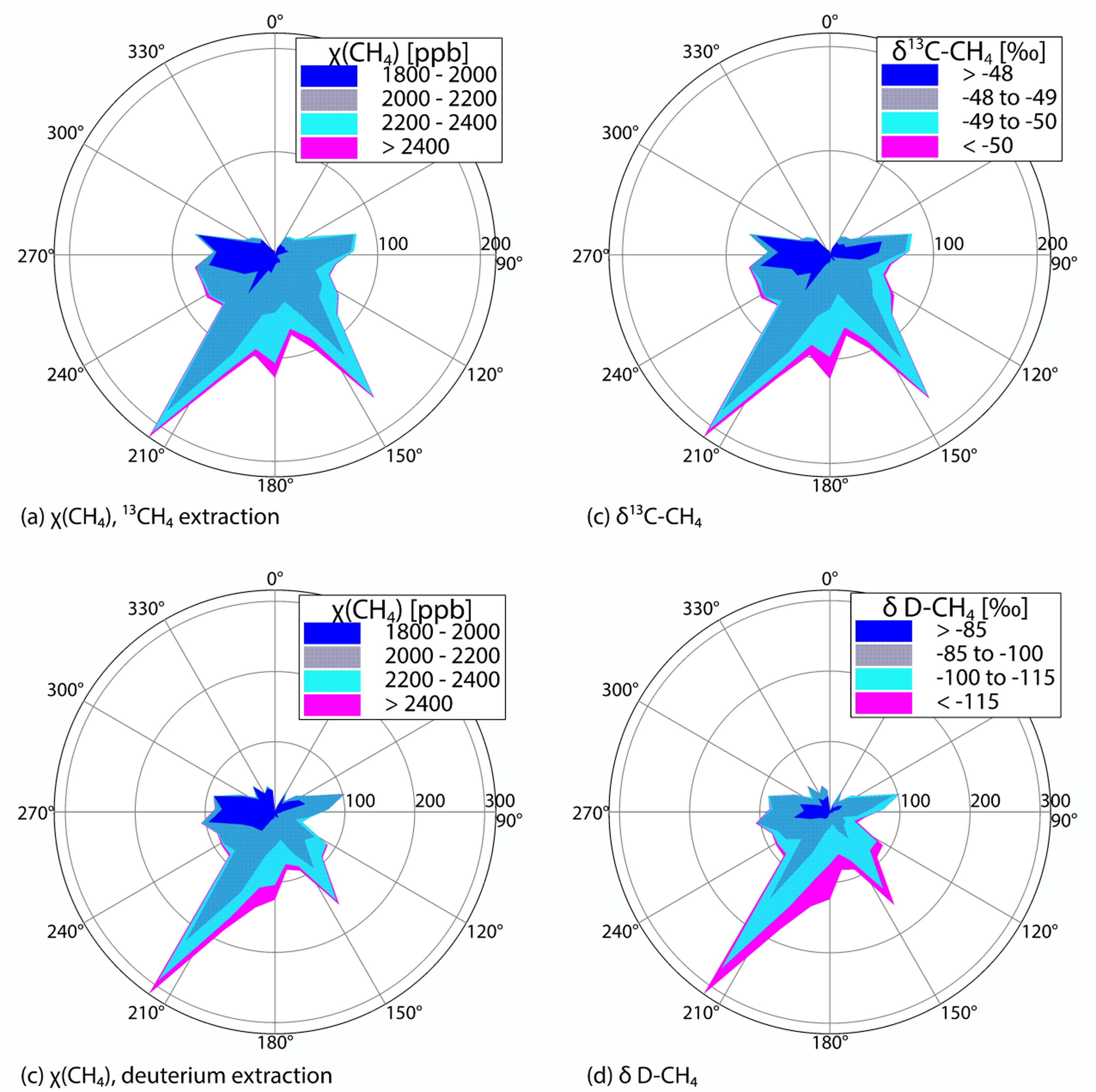
Fig. 3.
Wind rose diagrams of χ(CH4), δ 13C-CH4, and δD-CH4, in number of records with respect to the wind direction. The North is set at 0°, as for all the direction angles throughout the article.
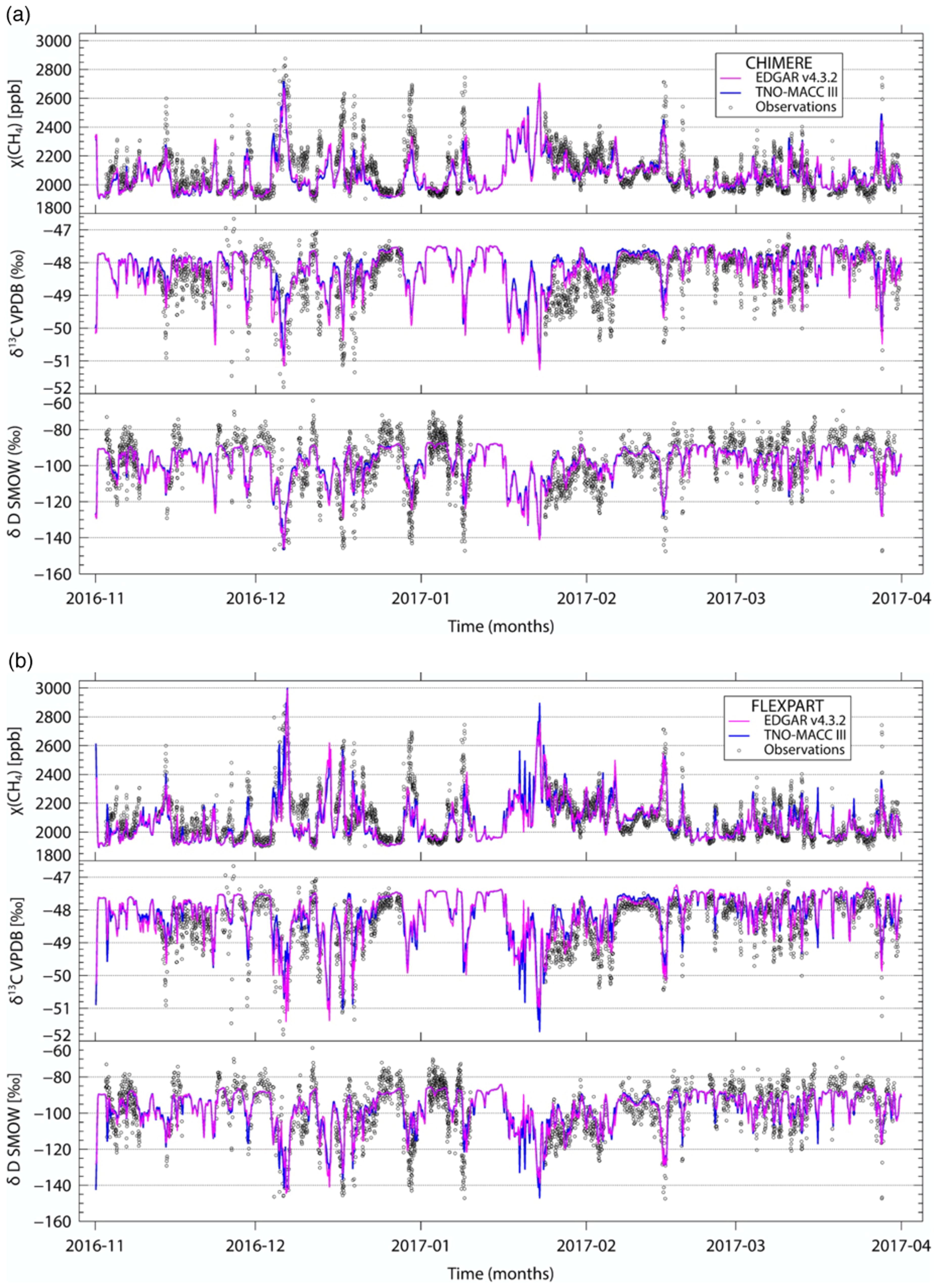
Fig. 4.
Model results from CHIMERE and FLEXPART-COSMO, using two emission inventories.
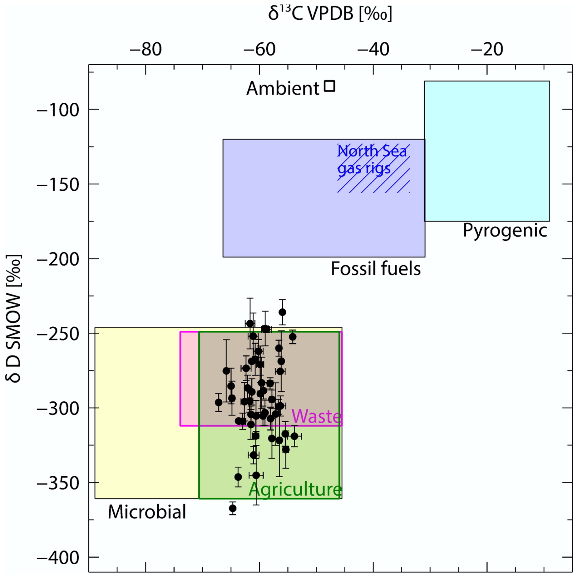
Fig. 5.
δ 13C- and δD-CH4 source signatures, derived with the moving window Keeling plot approach (black dots). The background CH4 isotopic composition corresponds to the 10th lower percentile of the χ(CH4) in this study’s dataset. Colored areas indicate typical isotope signatures for CH4 (referred in Table 1 and partially from unpublished measurements of biogenic sources made in the Netherlands). The δ 13C of the North Sea gas rigs is between −32 and −45‰, from Hitchman, S. P. (1989), Cain et al. (2017) and Riddick et al. (2019).
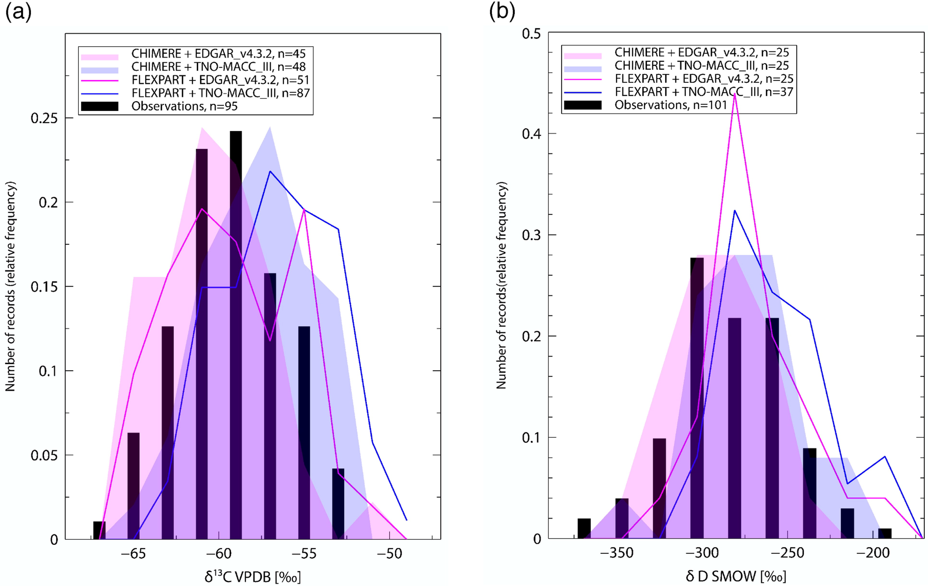
Fig. 6. Frequency distribution of the δ 13C and δD source signatures derived from the moving window Keeling plot approach applied to the observation and modelled time series, interpolated linearly to the measurement times. Signatures from the same peak were averaged to give one value per pollution event.
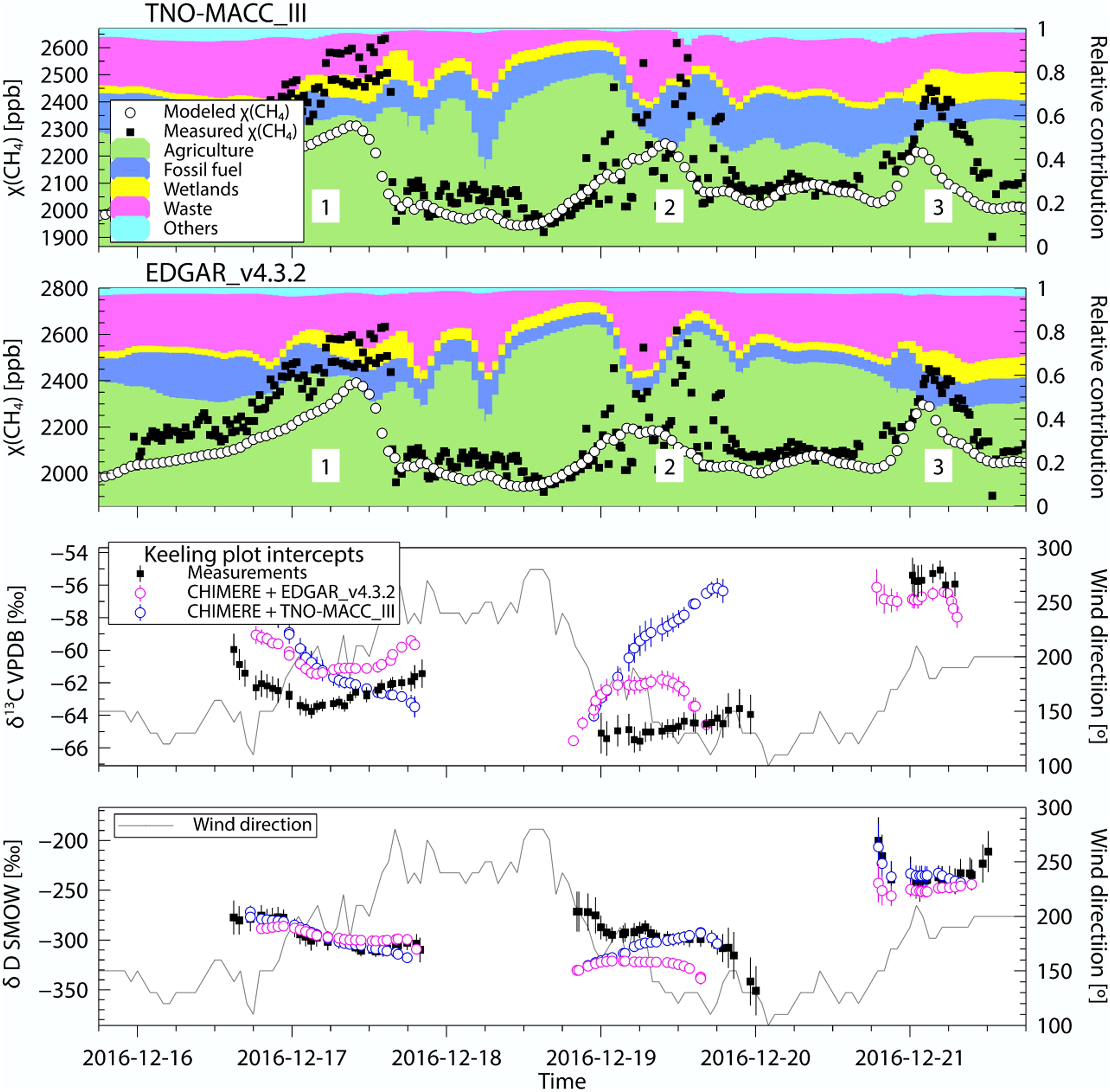
Fig. 7.
December 16 to 21 subset. The upper panels show χ(CH4) time series with an average time resolution of 51 min for the observations and 1 h for the model (left axis), with the modelled source partitioning (right axis). The lower panels show source signatures resulting from the moving window Keeling plot (left axis) with the recorded wind directions (right axis).
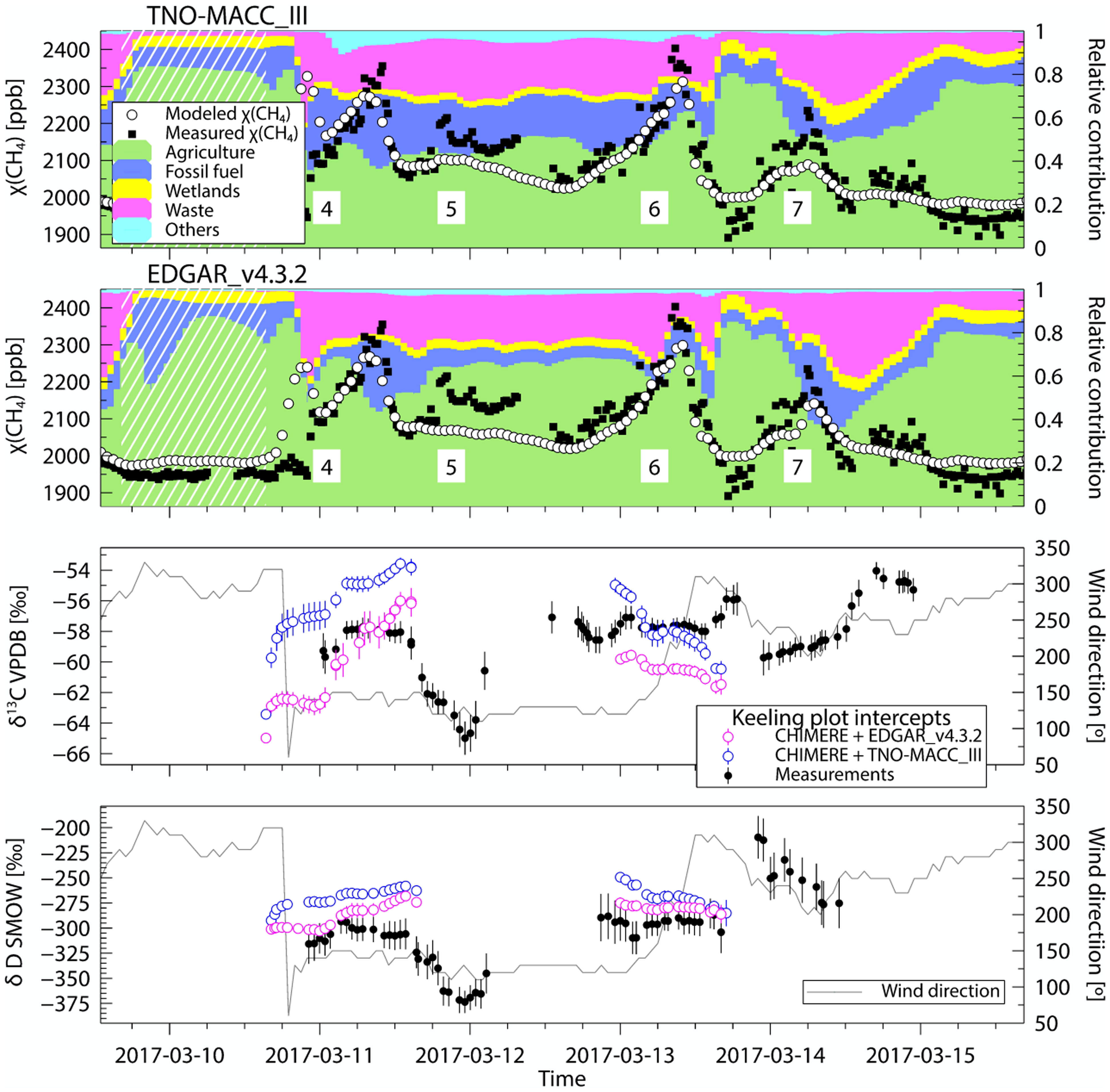
Fig. 8.
March 10 to 15 subset. The upper panels show χ(CH4) time series with an average time resolution of 51 min for the observations and 1 h for the model (left axis), with the modelled source partitioning (right axis). The lower panels show source signatures resulting from the moving window Keeling plot (left axis) with the recorded wind directions (right axis). The white hatching shows stable background χ(CH4) advected by northern winds.
Table 3.
Comparison of the averaged source signatures obtained from the Cabauw and Lutjewad time series. The values (y-intercept in [‰] ± 1σ) are obtained from a weighted orthogonal distance regression (ODR) minimising the sum of squared weighted orthogonal distances of all the data points to the fitted curve.
Table 4.
Comparison of the averaged source signatures from measurements and models. They correspond to the Keeling plot intercepts using all data. The values (y-intercept in [‰] ± 1σ) are obtained from a weighted orthogonal distance regression (ODR) minimising the sum of squared weighted orthogonal distances of all the data points to the fitted curve.
Table 1. Initial δ 13C and δD values from literature used in the models for the different emission sectors (Szénási 2019). They are derived from signatures found in the cited studies. The range of values is reported in the brackets. Only the δ 13C value for fossil fuel emissions (bold) was modified from Szénási 2019 to better represent the emissions from this sector in the Netherlands.
[−361; −295]Uzaki et al., 1991; Levin et al., 1993; Tyler et al., 1997; Bréas et al., 2001; Bilek et al., 2001; Klevenhusen et al., 2010; Röckmann et al., 2016Waste−55 [−73.9; −45.5]−293
[−312; −293]Games and Hayes, 1976; Levin et al., 1993; Bergamaschi et al., 1998; Zazzeri et al., 2015; Röckmann et al., 2016Extraction and distribution of fossil fuels & non-industrial combustion−40.0 [−66.4; −30.9]−175
[−199; −175]Levin et al., 1999; Lowry et al., 2001; Thielemann et al., 2004; Zazzeri et al., 2016; Röckmann et al., 2016Other anthropogenic sources−35.0 [−60; −9]−175
[−175; −81]Levin et al., 1999; Chanton et al., 2000; Nakagawa et al., 2005; Röckmann et al., 2016Natural wetlands−69 [−88.9; −51.5]−330 [−358; −246]Tyler et al., 1987; Smith et al., 2000; Galand et al., 2010; Happell et al., 1995; Martens et al., 1992; Bilek et al., 2001; Sugimoto and Fujita, 2006