
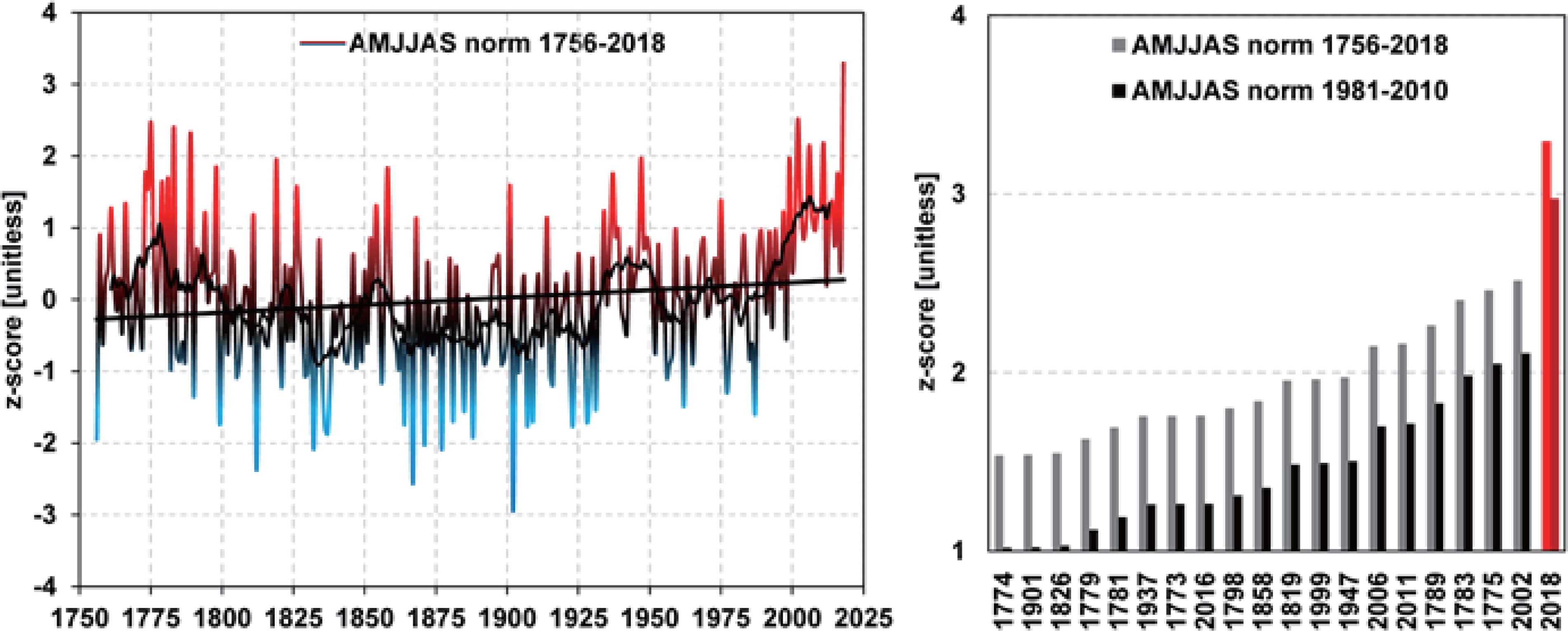
Fig. 1.
Annual mean warm-season temperatures (April to September) in Stockholm 1756–2018. Left: Time evolution and long-term trend of warm-season temperatures normalized relative to the mean of 1756–2018. Right: Ranked warm seasons >1 z-score relative to 1756–2018 (grey) and their z-scores relative to 1981–2018 (black). The data was corrected for urban heat island effect (Moberg et al., 2002a). The linear warming trend is significantly different from zero at p<0.01. Data by A. Moberg is taken from the Bolin Centre Database https://bolin.su.se/data/.
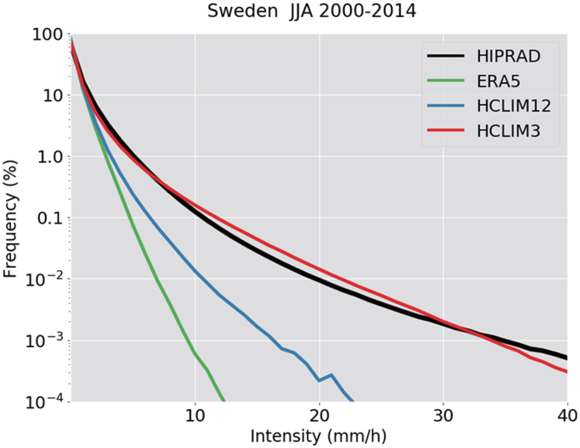
Fig. 2.
Frequency diagram showing summer (June-August) hourly precipitation from all model grid points in Sweden. HIPRAD is a combined radar and rain gauge data set covering Sweden at 2 × 2 km at 1-hourly time resolution (Berg et al., 2016). ERA5 is the global reanalysis data at 30 km horizontal resolution (Hoffmann et al., 2019) used to force the regional climate models at 12 km (HCLIM12) and 3 km (HCLIM3). All model results have been calculated at their native grid resolution and only data from events with > 0.1 mm/hour has been included. The figure clearly shows higher precipitation intensities with higher model resolution that is closer to the observations..
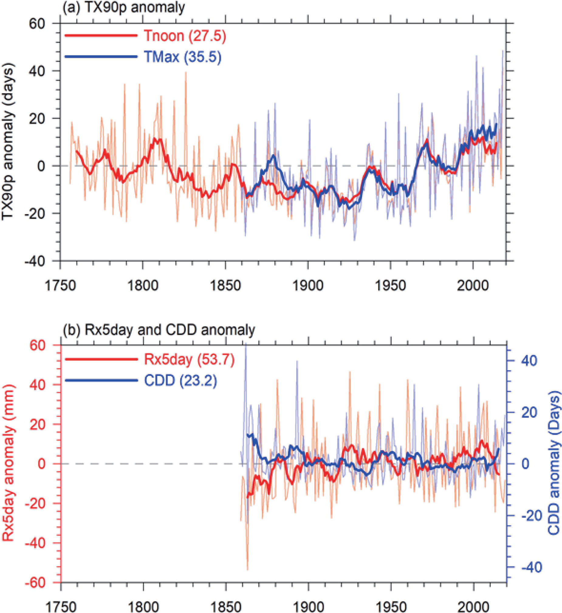
Fig. 3.
Time series of (a) anomalies of TX90p (number of days when daily maximum temperature (TMax) > 90th percentile) during 1756–2018, (b) anomalies of R × 5day (maximum consecutive 5-day precipitation) and CDD (maximum number of consecutive days with daily precipitation amount < 1mm) during 1859–2018, with reference period 1961–1990, for Stockholm. Thick lines show the 9-years running average of the time series. Daily temperature and precipitation data for Stockholm were provided by Moberg et al. (2002a) (Same as Figure 1) and SMHI (downloaded from https://opendata.smhi.se/). Since there was no TMax observation during 1756–1858, the noon (13–14 PM CET) observation of the three times per day observations of temperature was taken as a proxy for Tmax in the calculation of TX90p during 1756–1858. The two curves of TX90p using Tmax and the noon observation during 1859–2018 generally follow each other well, which makes the longer perspective by extending the data back to 1756 meaningful and interesting. Values in the brackets show the climatological means during 1961–1990 for each index..
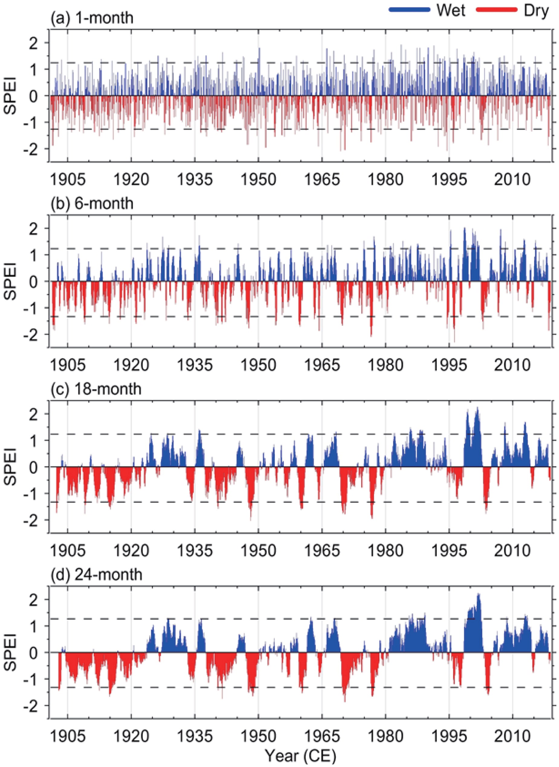
Fig. 4.
Multi-timescale monthly SPEI variability in Sweden over 1901–2018. (a) 1-month SPEI from 1901-01 to 2018–12; (b) 6-month SPEI from 1901–06 to 2018-12; (c) 18-month SPEI from 1902-06 to 2018-12; (d) 24-month SPEI from 1902-12 to 2018-12. Upper and lower horizontal dashed lines in each panel indicate 95th and 5th percentile of SPEI over the whole time period, respectively. The SPEI calculations are based on CRU TS v.4.03 monthly precipitation and potential evapotranspiration 0.5 longitude × 0.5 latitude grid dataset (Harris et al. 2014), which is accessible from http://dx.doi.org/10.5285/10d3e3640f004c578403419aac167d82.