
Table 1.
List of observed properties, deployed instrumentation and consequent nomenclature adopted in the present study. The operational time resolution of both trace gas and aerosol measuring instruments was of 1 second.
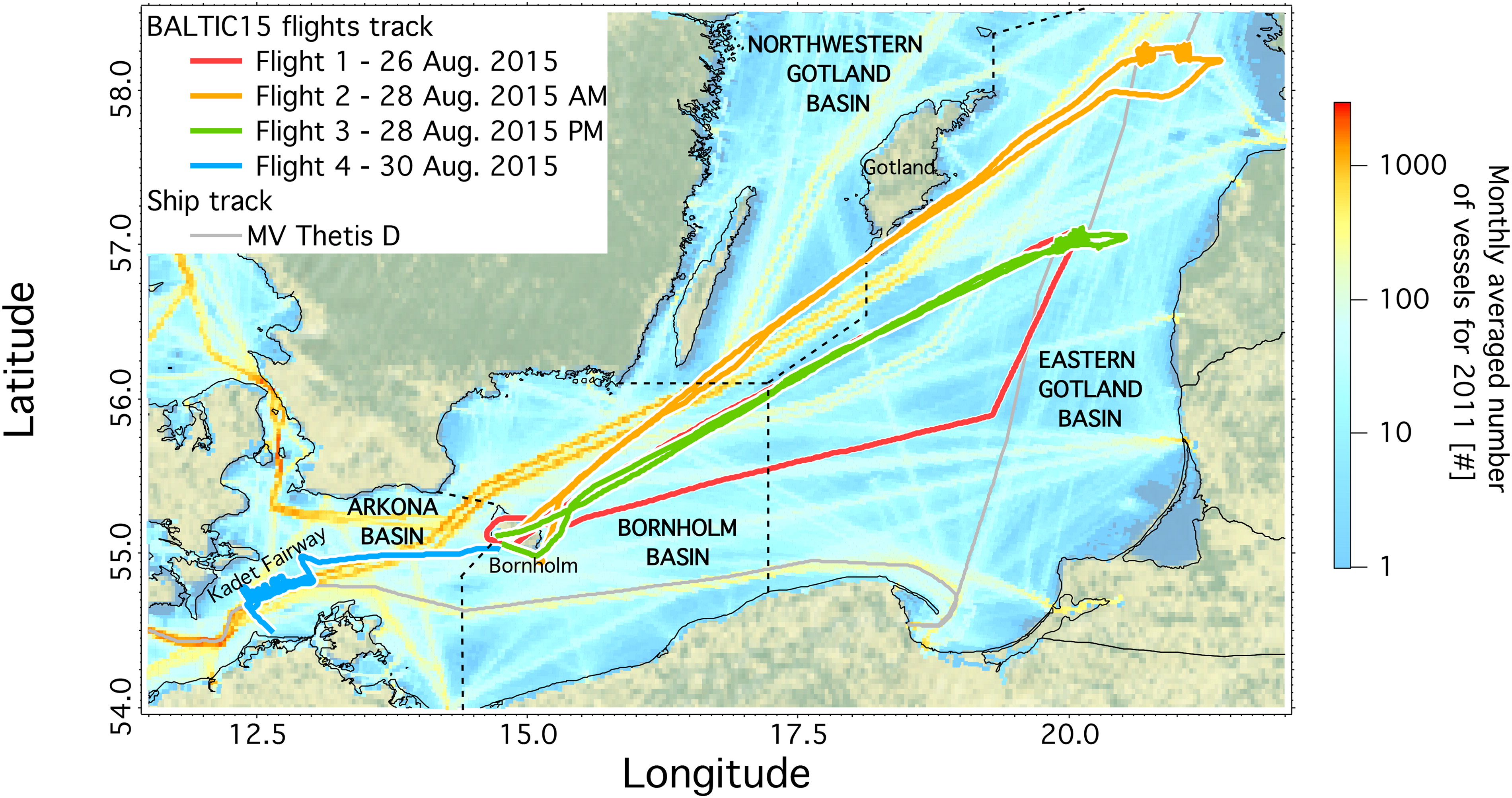
Figure 1.
Map of the Baltic Sea including vessels density for 2011 (HELCOM) and the flight patterns of the AWI research aircraft Polar 5 during the BALTIC’15 campaign. The grey line represents the track of the cargo vessel “Thetis D”.
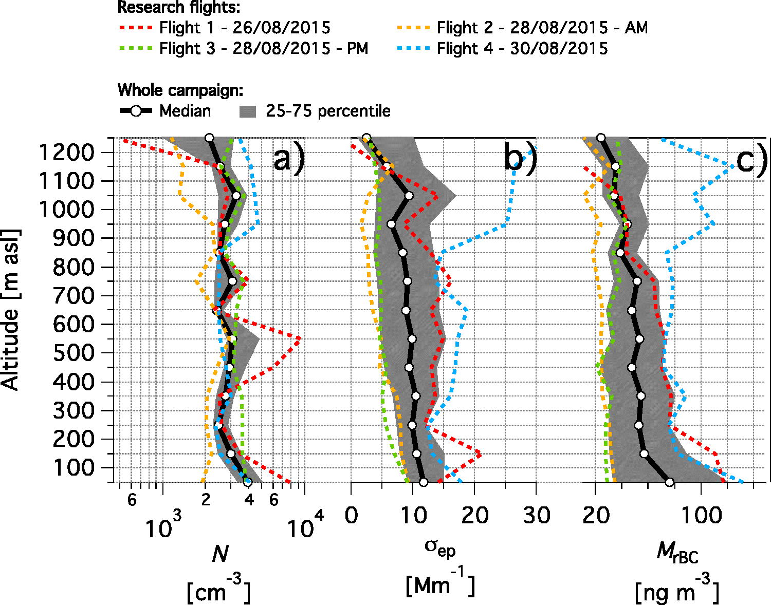
Figure 2.
Vertical profiles of each single flight and whole campaign for: (a) aerosol number concentration of particle with diameter larger than 13 nm (N); (b) aerosol extinction coefficient measured at 630 nm (σ ep); (c) rBC mass concentration of rBC particles with a diameter between 80-700 nm (M rBC). Statistics calculated for equidistant altitude steps starting at the surface (0 m asl) and 100 m thick.
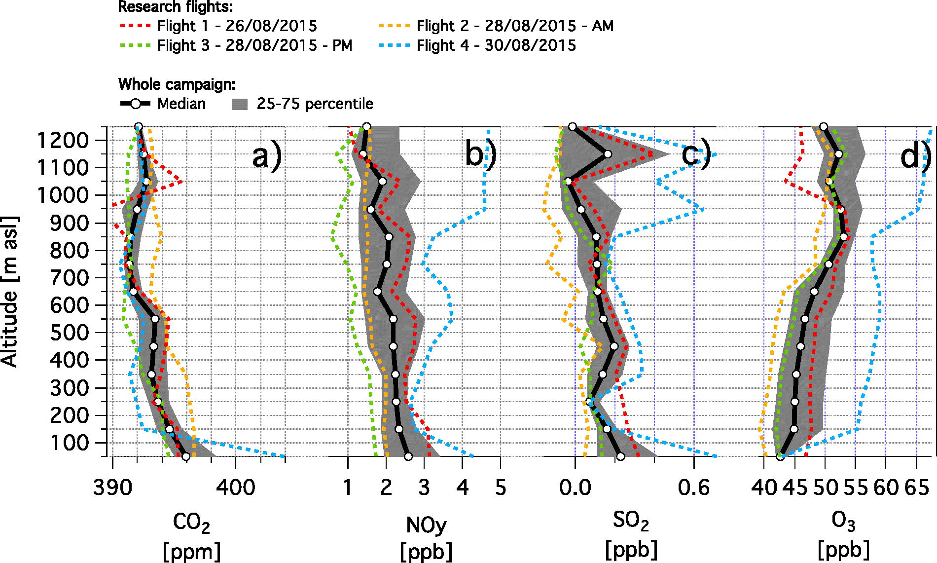
Figure 3.
Vertical profiles of each single flight and whole campaign for mixing ratios of: (a) carbon dioxide (CO2); (b) reactive nitrogen compounds (NOy ); (c) sulphur dioxide (SO2); (d) ozone (O3). Statistics calculated for equidistant altitude steps starting at the surface (0 m asl) and 100 m thick.
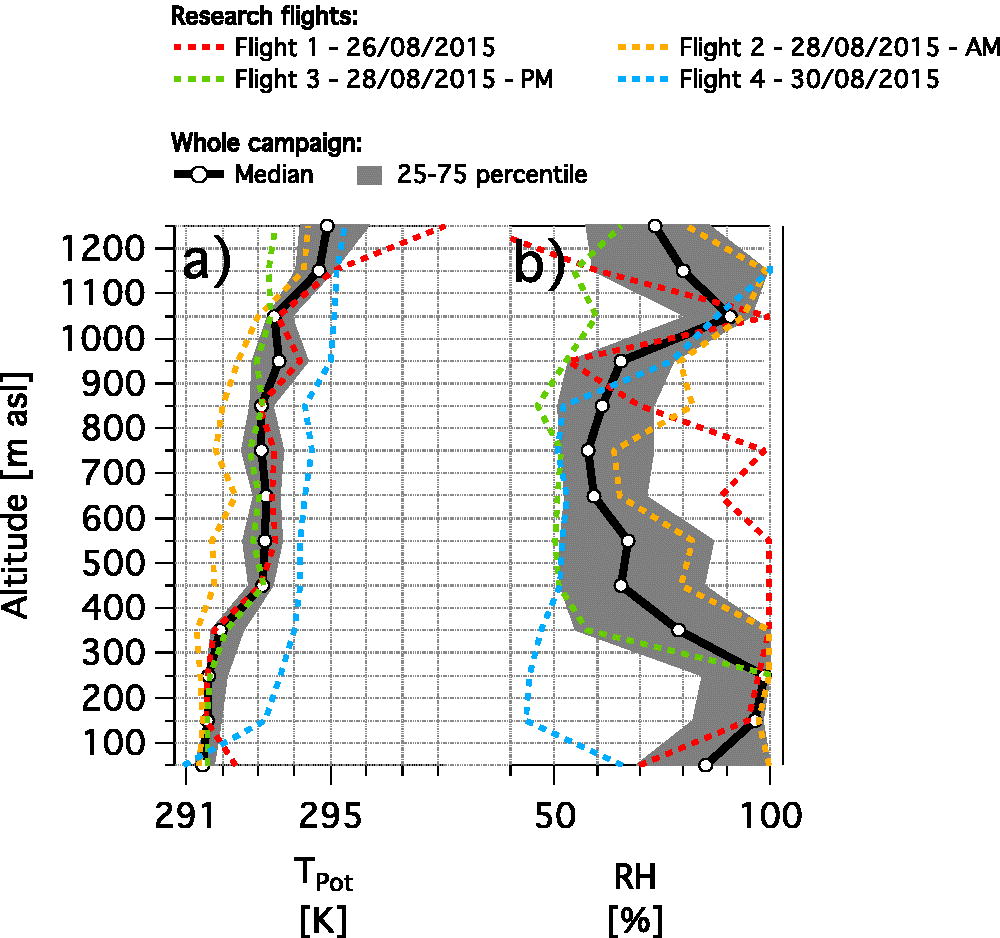
Figure 4.
Vertical profiles of each single flight and whole campaign for: (a) Potential temperature (TPot); (b) Relative humidity (RH). Statistics calculated for equidistant altitude steps starting at the surface (0 m asl) and 100 m thick.
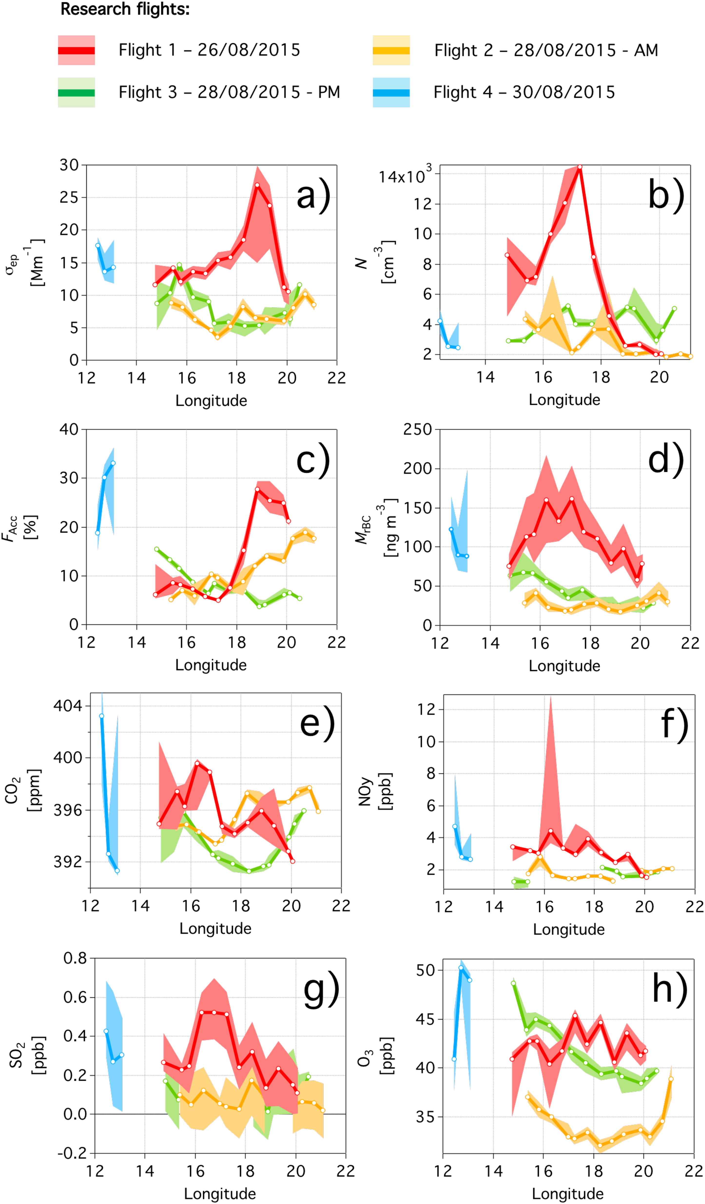
Figure 5.
Longitudinal variability in the marine boundary layer (altitude below 400 m asl) of: (a) aerosol extinction coefficient measured at 630 nm (σep); (b) aerosol number concentration of particle with diameter larger than 13 nm (N); c) aerosol number fraction of accumulation particles having diameter between 100-1000 nm (F Acc) d) mass concentration of black carbon particles with a diameter between 80-700 nm (M rBC); e) CO2 mixing ratio; (f) NOy mixing ratio; (g) SO2 mixing ratio; (h) O3 mixing ratio. Median and 25-75 % percentiles calculated with 0.5 degrees resolution and displayed as line and shadow, respectively.
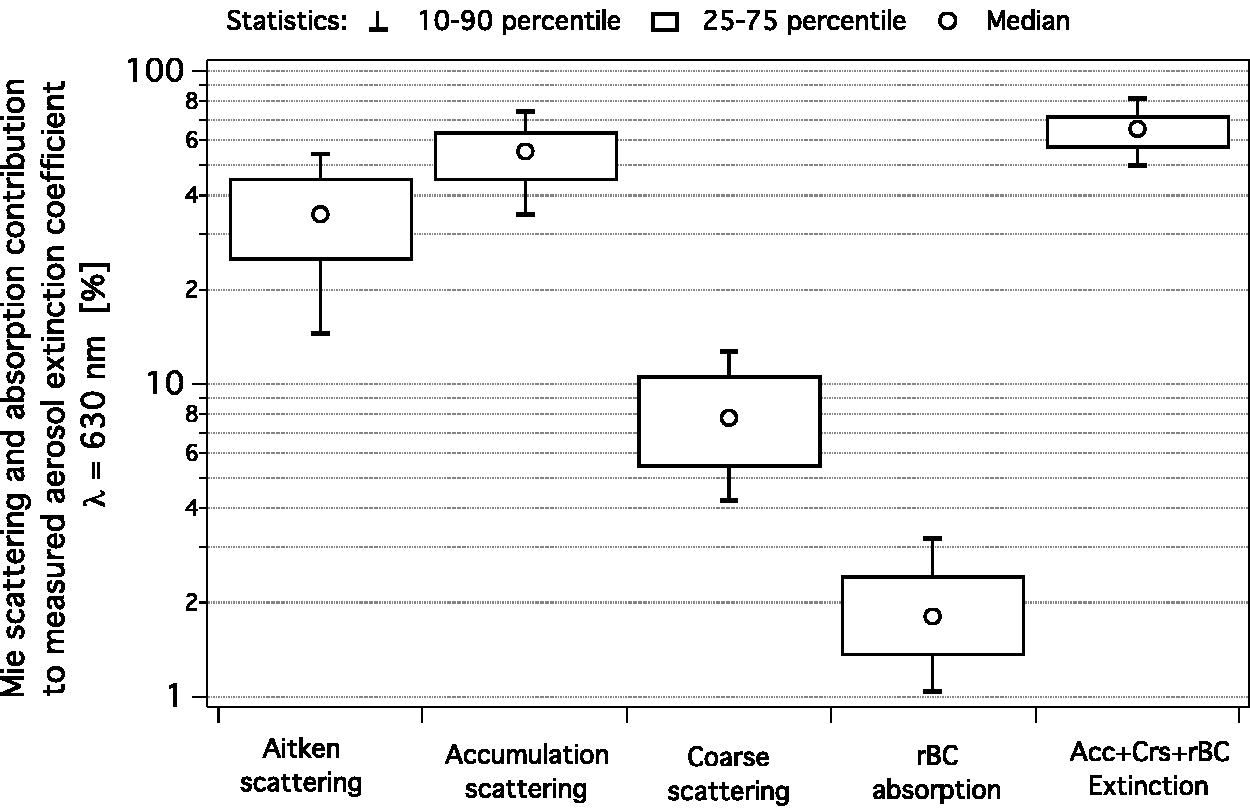
Figure 6.
Relative contribution of different aerosol types to the extinction coefficient observed in the marine boundary layer (altitude below 400 m asl): scattering of Aitken, accumulation and coarse mode particles; absorption of BC particles; extinction of accumulation-coarse-rBC particles. Percentage contributions to extinction are calculated as the ratio of scattering-absorption-extinction of the different aerosol components estimated with Mie theory over the extinction coefficient observed with the CAPS at a wavelength of 630 nm. Absolute scattering and absorption coefficient are calculated with Mie theory from the observed total aerosol and rBC size distributions, respectively. Aitken particles: diameter between 10-100 nm; accumulation particle diameter between 100-1000 nm; coarse particle diameter between 1000-2500 nm; rBC particle diameter between 80-700 nm.
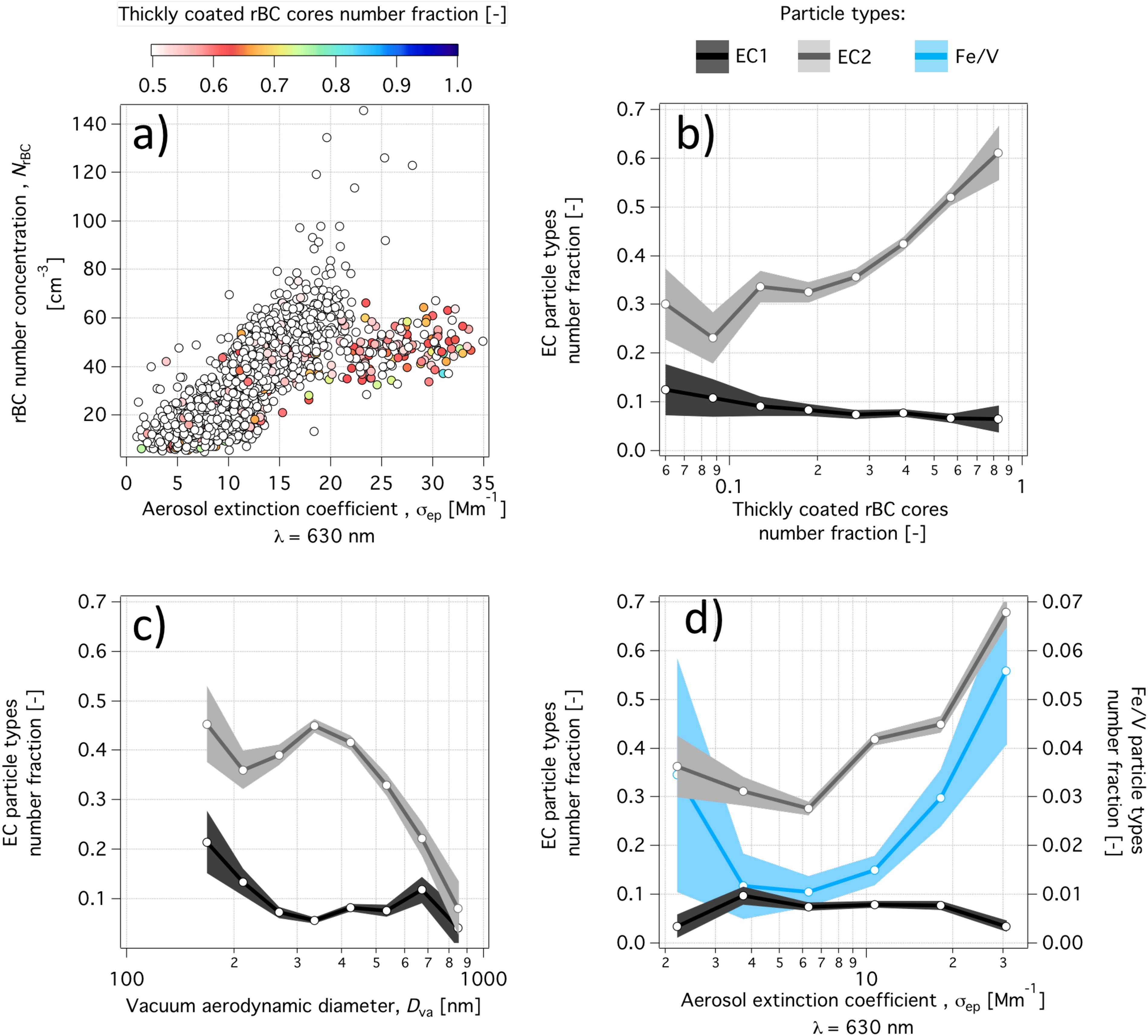
Figure 7.
Aerosol chemical composition measured by the ALABAMA and rBC mixing measured by the SP2 in the marine boundary layer at altitude below 400 m asl during the whole BALTIC’15 campaign: (a) Comparison between the rBC number concentration measured with the SP2 with the aerosol extinction observations at 630 nm; (b) Comparison between the particle number fractions of EC1 and EC2 types detected with the ALABAMA and the fraction of thickly coated rBC particles quantified with the SP2; (c) Size distribution of EC1 and EC2 particle types; (d) Comparison of the aerosol extinction observations at 630 nm with the particle number fractions of EC1, EC2, and Fe/V types. The particle types fraction was calculated as the number of the identified components normalized to the total number of particles analysed by the ALABAMA. ALABAMA uncertainties, based on binomial statistics, are shown as shadow.
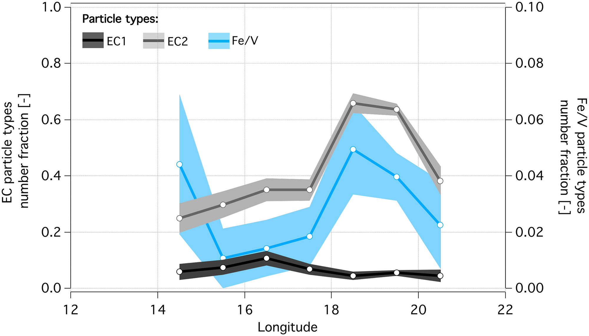
Figure 8.
Longitudinal variability with 1-degree resolution of the single particle chemical composition measured by the ALABAMA in the marine boundary layer observed during Flight 1 on 26 August 2015. Fractions are normalized to the total number of particles detected by the ALABAMA. Uncertainties based on binomial statistics are shown as shadow.
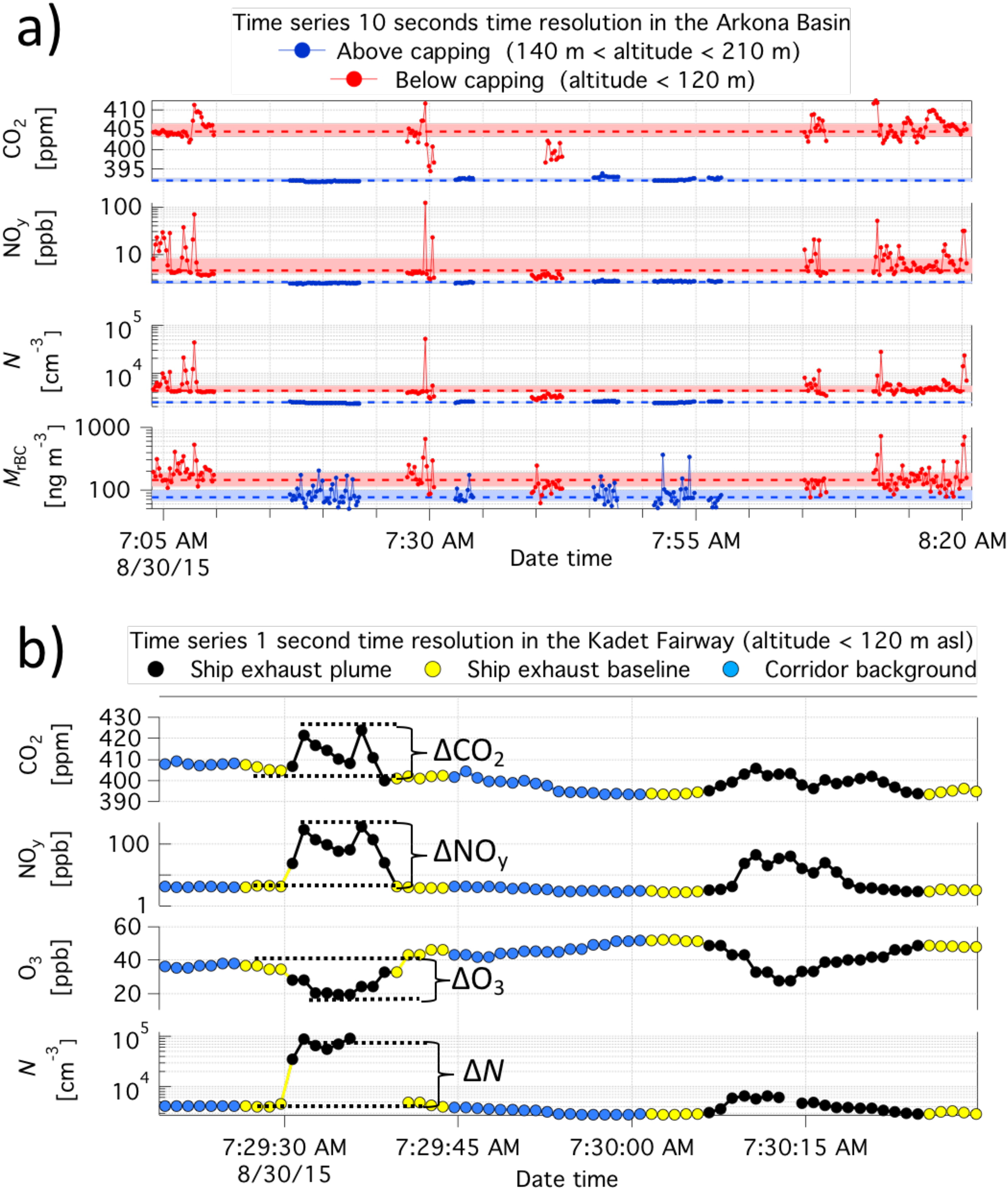
Figure 9.
Time series of Flight 4 occurred on 30 August 2015 in the Arkona Basin. (a) Time series with 10 seconds time resolution of trace gases and aerosol particles used for the identification of two atmospheric layers separated by a capping at approximately 120 m asl. Dotted line and shading represent the median and interquartile range, respectively. (b) Example of single ship exhaust peaks sampled below capping (< 120 m asl) in the shipping corridor "Kadet Fairway" (1 second time resolution). N: number concentration of particle with diameter larger than 13 nm; M rBC: rBC mass concentration of rBC particles with a diameter between 80-700 nm.
Table 2.
Statistics of the aerosol and gas concentration-property observed during Flight 4 occurred on 30 August 2015 in the Arkona Basin. First two columns: median values for air sampled in the ship exhaust and in the corridor background. Third column: enchantment ratio (unit less) calculated as the ratio of ship exhaust median over corridor background median.
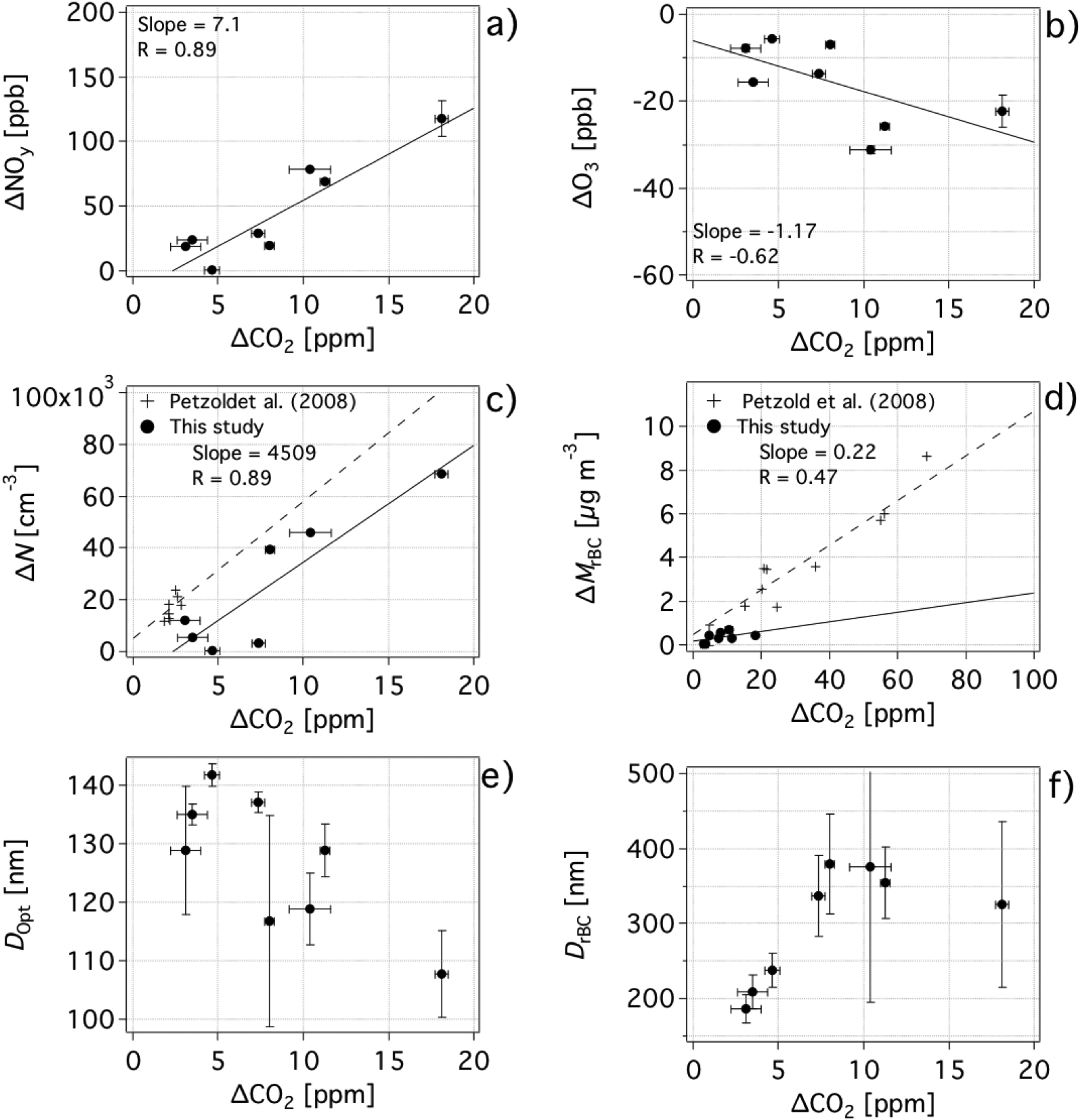
Figure 10.
Scatter plot of different exhaust species over the CO2 excess (ΔCO2) for the specific ship plumes observed in the "Kadet Fairway". (a) Reactive nitrogen compounds excess (ΔNOy); (b) ozone excess (ΔO3); (c) number concentration excess of particles with diameter larger than 13 nm (ΔN); (d) mass concentration excess of black carbon particles with diameter between 80-700 nm (ΔM rBC); (e) total particles number mean diameter (D Opt); (f) black carbon mass mean diameter (D rBC). Standard deviation represented as error bars.
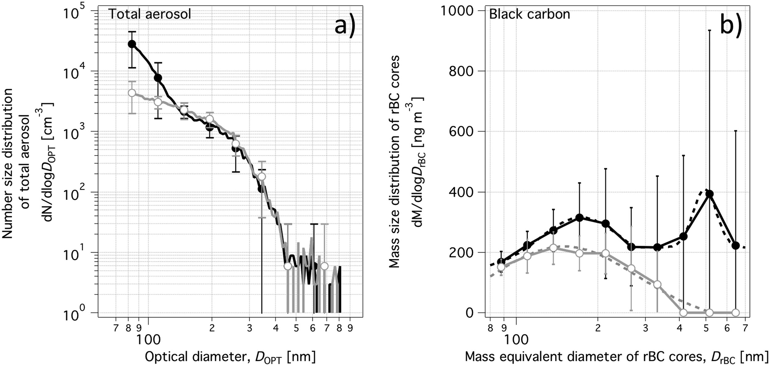
Figure 11.
Averaged mass size distribution observed in fresh ship plumes (ΔCO2>10 ppm) and in more diluted plumes (ΔCO2<5 ppm) for (a) total aerosol particles measured with the UHSAS and (b) refractory black carbon cores measured with the SP2. Standard deviation displayed as error bars and lognormal fit (only for refractory black carbon) as dotted line.