
Table 1.
Comparison of Particle Collection Efficiencies for Vegetation Canopies from Selected Algorithms.
[i] = a characteristic length scale for canopy element interception in Zhang et al. (2001) (m).
[ii] = a characteristic width of the “small” and “large” interception collectors, respectively in Slinn (1982) (m).
[iii] = numerical constant in rebound expression – Slinn (1982) recommended = 2.
[iv] = LUC-specific coefficient in Brownian collection efficiency expression of Petroff and Zhang (2010).
[v] = LUC-specific coefficient in impaction collection efficiency expression of Petroff and Zhang (2010).
[vi] = LUC-specific coefficient in interception collection efficiency expression of Petroff and Zhang (2010).
[vii] = LUC-specific coefficient in turbulent impaction collection efficiency expression of Petroff and Zhang (2010).
[viii] = the ratio of the viscous drag coefficient to the total drag coefficient in Slinn (1982).
[xv] = the fraction of total interception collection occurring on ‘small’ collectors (i.e. vegetation hairs) in the canopy in Slinn (1982).
[xvi] = LUC-specific characteristic length in Petroff and Zhang (2010) (m).
[xxi] = LUC-specific parameter used in the impaction collection efficiency expression of Zhang et al. (2001).
[xxii] = LUC-specific parameter used in the impaction collection efficiency expression of Petroff and Zhang (2010).
[xxiii] = LUC-specific exponent used in the Brownian collection efficiency expression of Zhang et al. (2001).
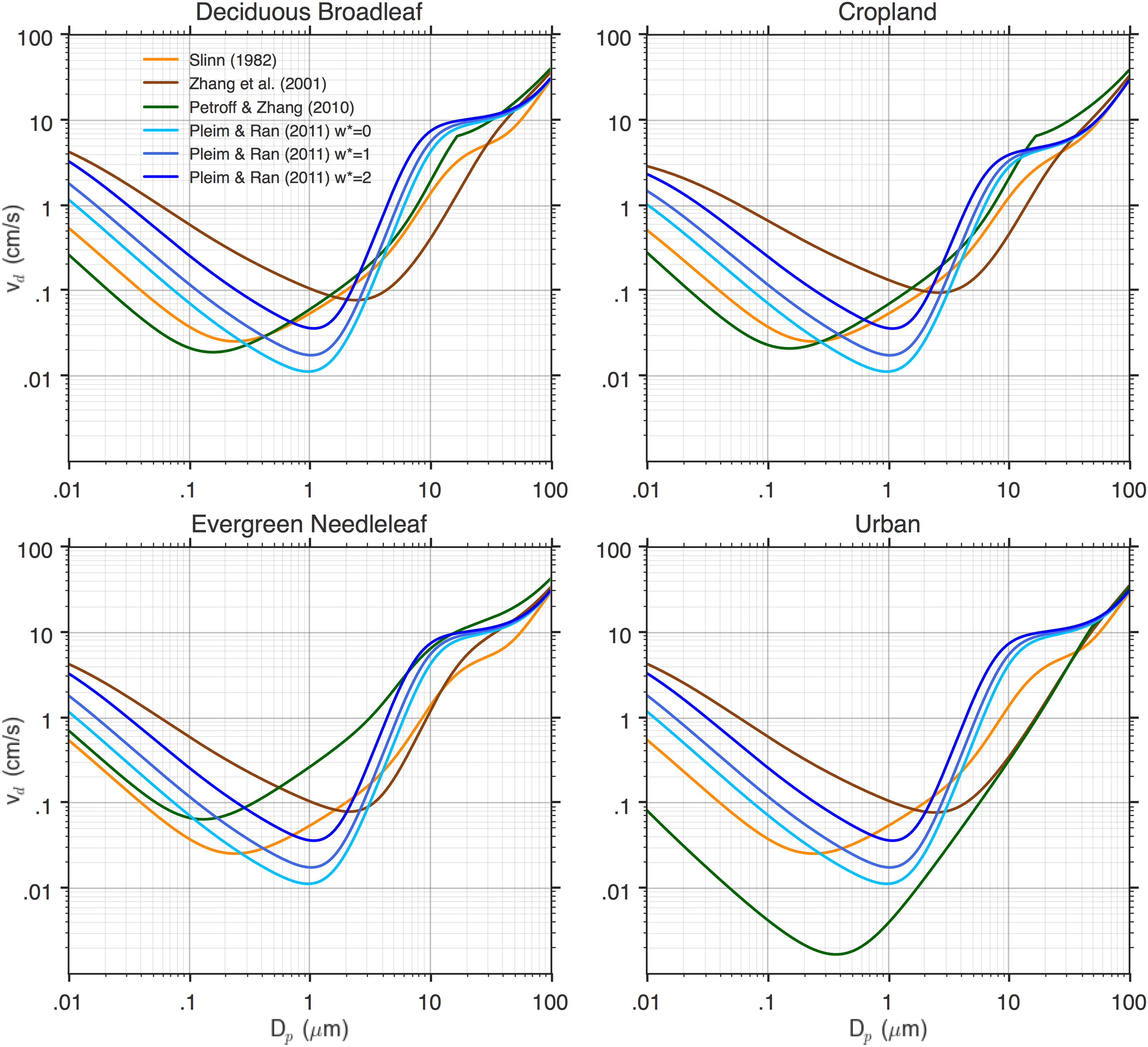
Fig. 1.
Comparison of particle dry deposition velocity, Vd (cm s−1), as a function of particle diameter, Dp (µm), for various algorithms and land use types (u* = 60 cm/s for all algorithms and LUCs).
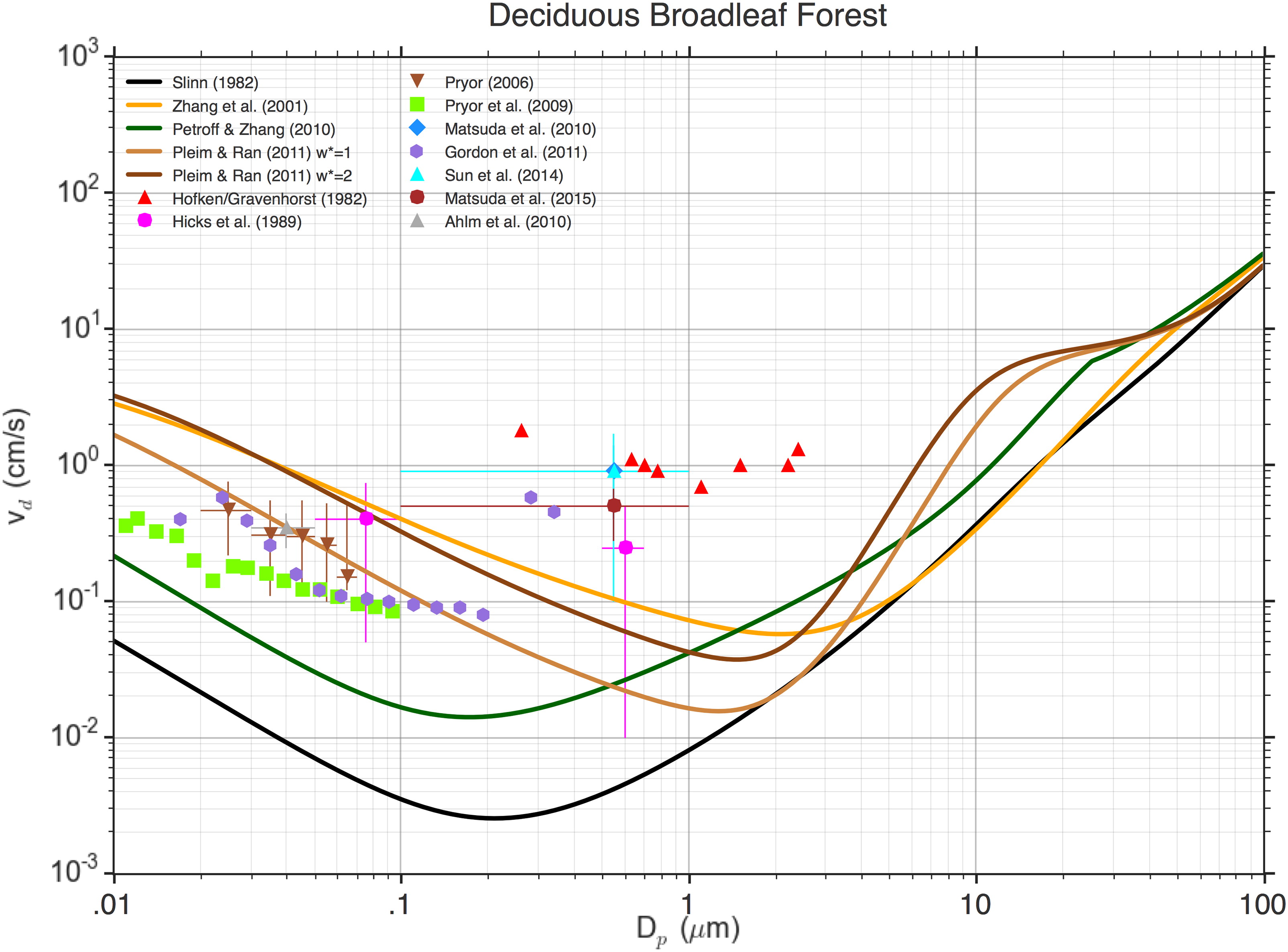
Fig. 2.
Atmospheric particle deposition velocities (cm s−1) predicted by the four algorithms compared with measurements as a function of particle diameter (µm) for a deciduous broadleaf forest. Error bars represent an estimate of uncertainty either as presented by the respective authors or as derived from the published data. (u* = 40 cm s−1 for all algorithms.).
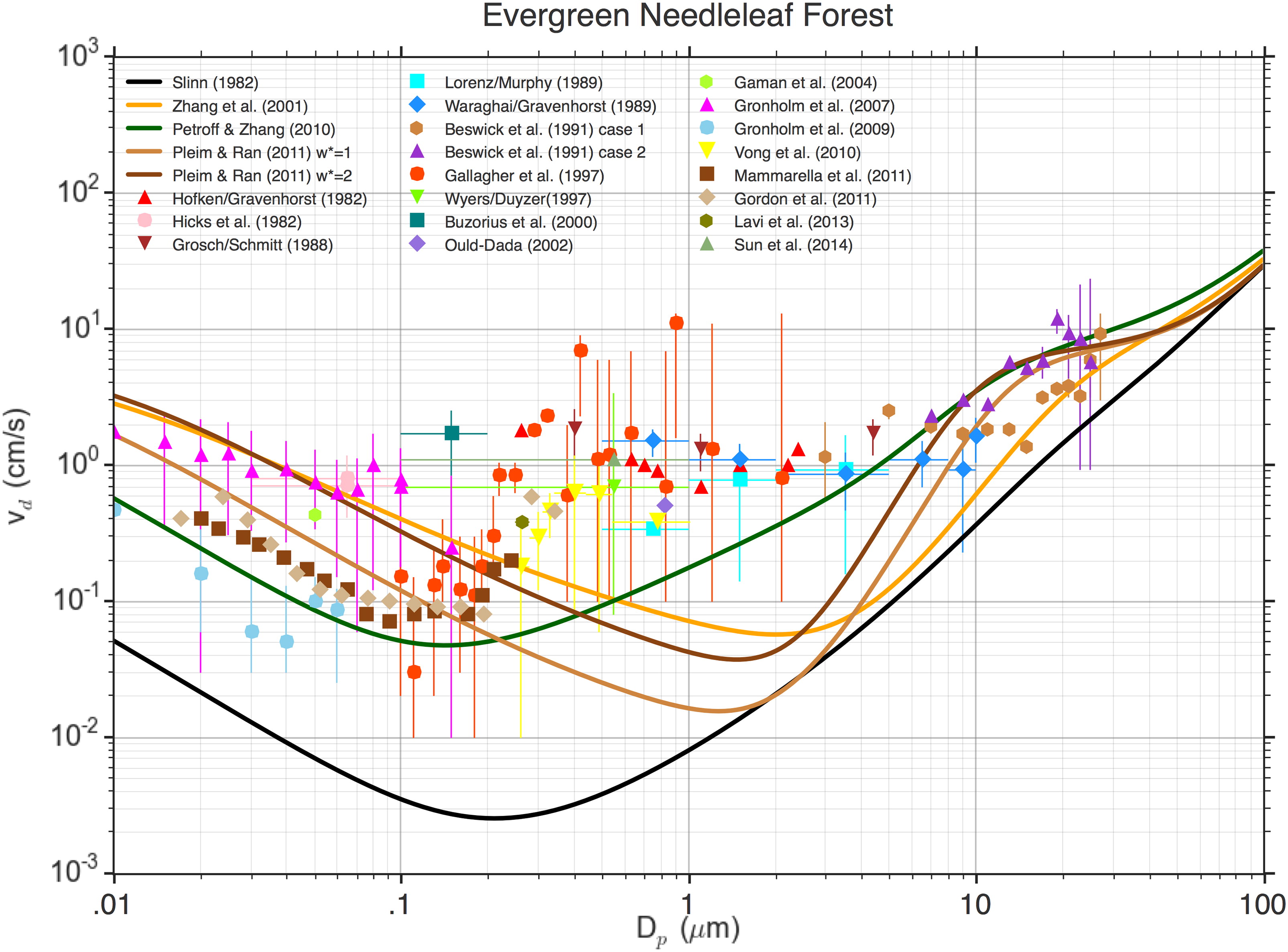
Fig. 3.
Atmospheric particle deposition velocities (cm s−1) predicted by the four algorithms compared with measurements as a function of particle diameter (µm) for a evergreen needleleaf forest. Error bars represent an estimate of uncertainty either as presented by the respective authors or as derived from the published data. (u* = 40 cm s−1 for all algorithms.).
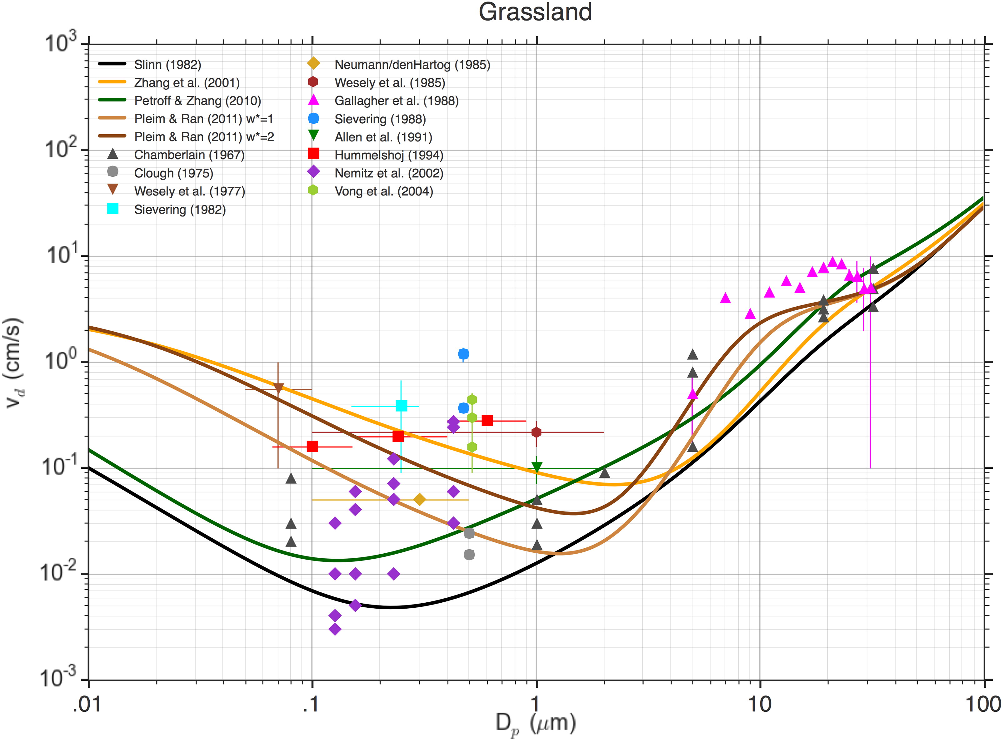
Fig. 4.
Atmospheric particle deposition velocities (cm s−1) predicted by the four algorithms compared with measurements as a function of particle diameter (µm) for a grass covered surface. Error bars represent an estimate of uncertainty either as presented by the respective authors or as derived from the published data. (u* = 40 cm s−1 for all algorithms.).
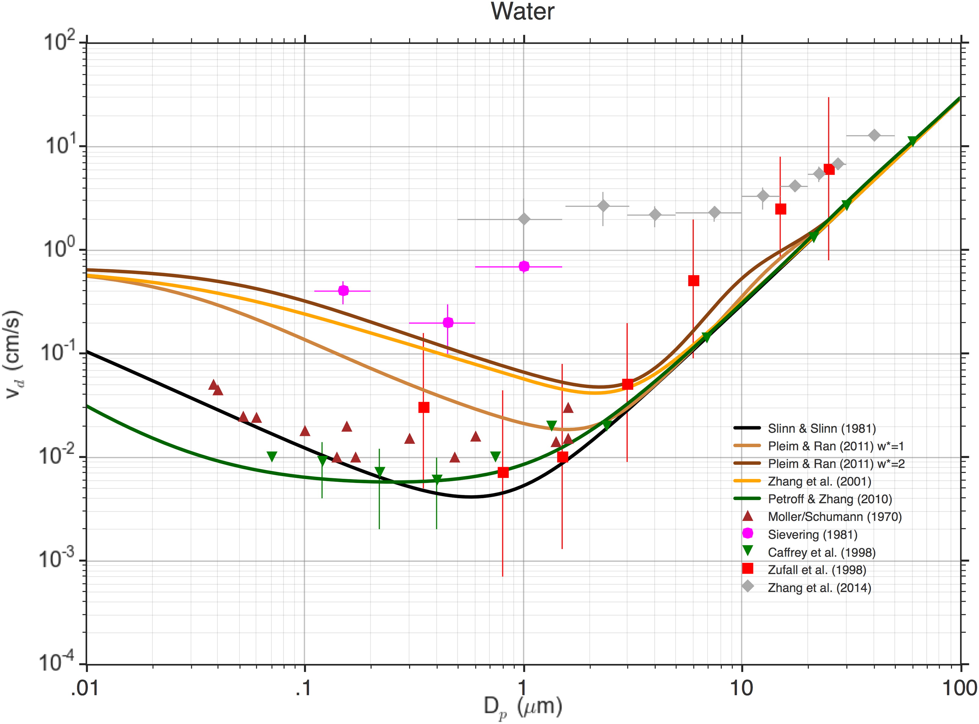
Fig. 5.
Atmospheric particle deposition velocities (cm s−1) predicted by the four algorithms compared with measurements as a function of particle diameter (µm) for a water surface. Error bars represent an estimate of uncertainty either as presented by the respective authors or as derived from the published data. (u* = 20 cm s−1 for all algorithms.).
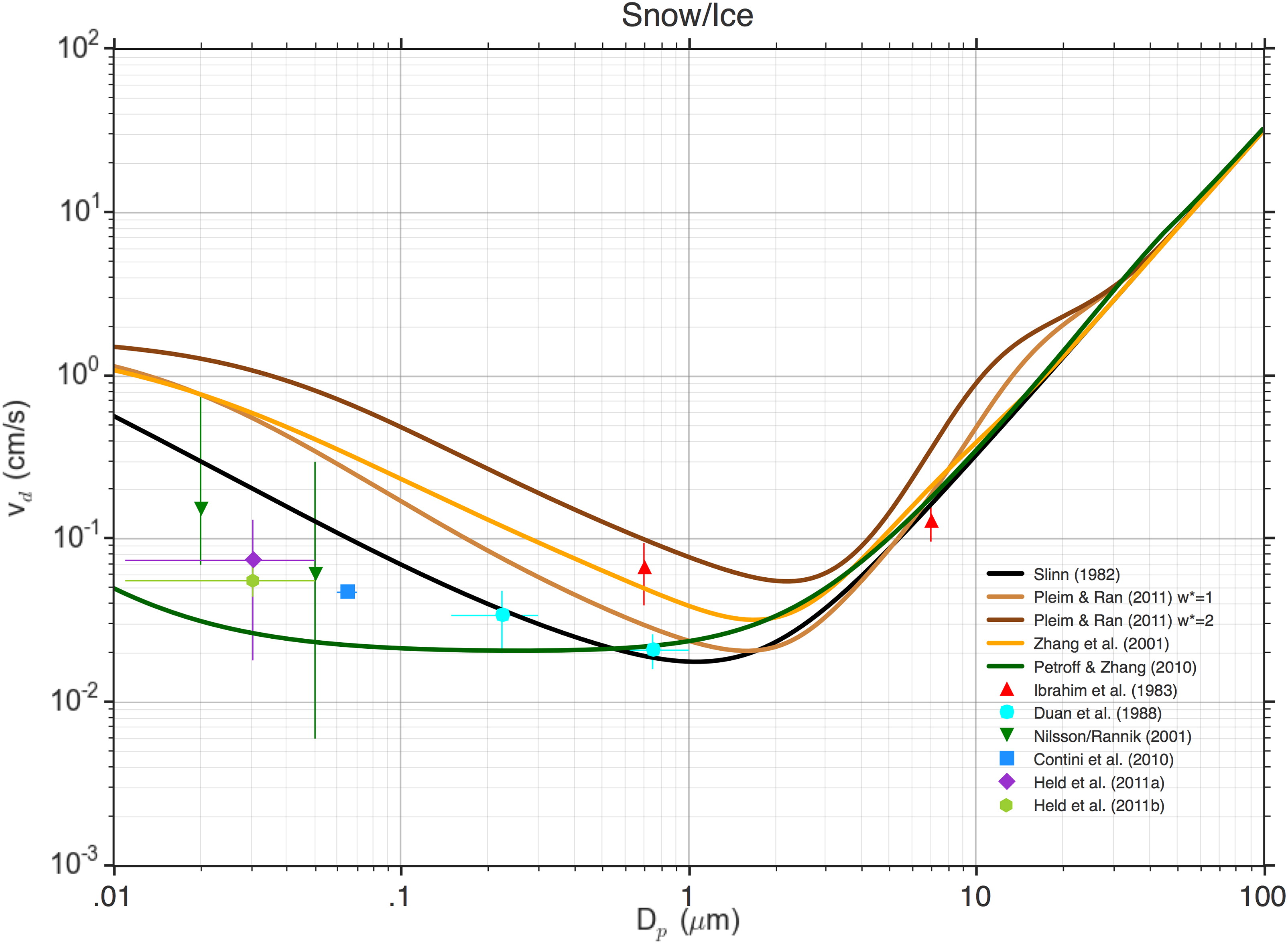
Fig. 6.
Atmospheric particle deposition velocities (cm s−1) predicted by the four algorithms compared with measurements as a function of particle diameter (µm) for a snow or ice covered surface. Error bars represent an estimate of uncertainty either as presented by the respective authors or as derived from the published data. (u* = 20 cm s−1 for all algorithms.).
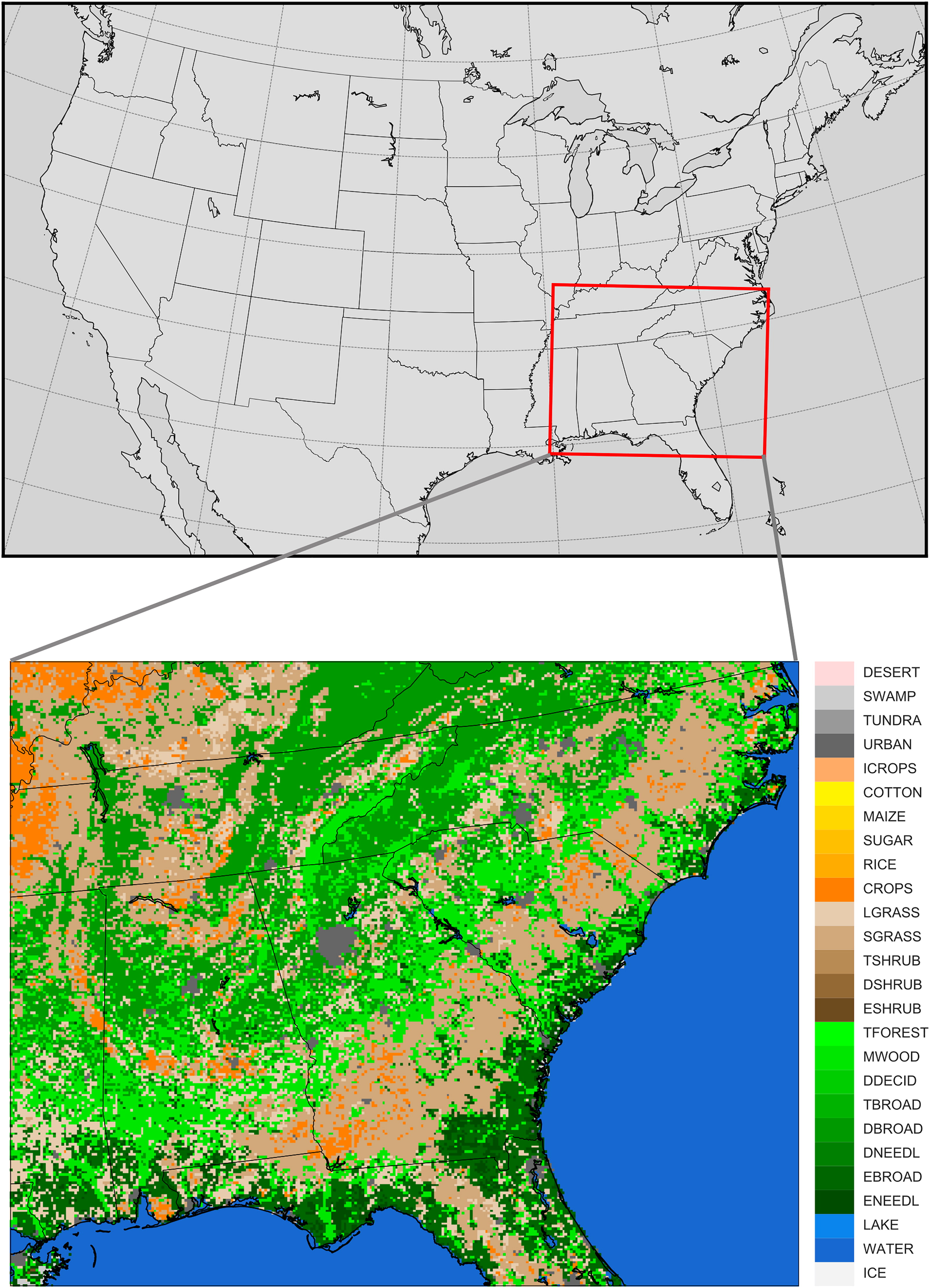
Fig. 7.
Computational domain consisting of the Southeastern domain (4 km horizontal resolution) nested within the CONUS domain (12 km horizontal resolution) used in the NOAA NWS National Air Quality Forecast Capability.
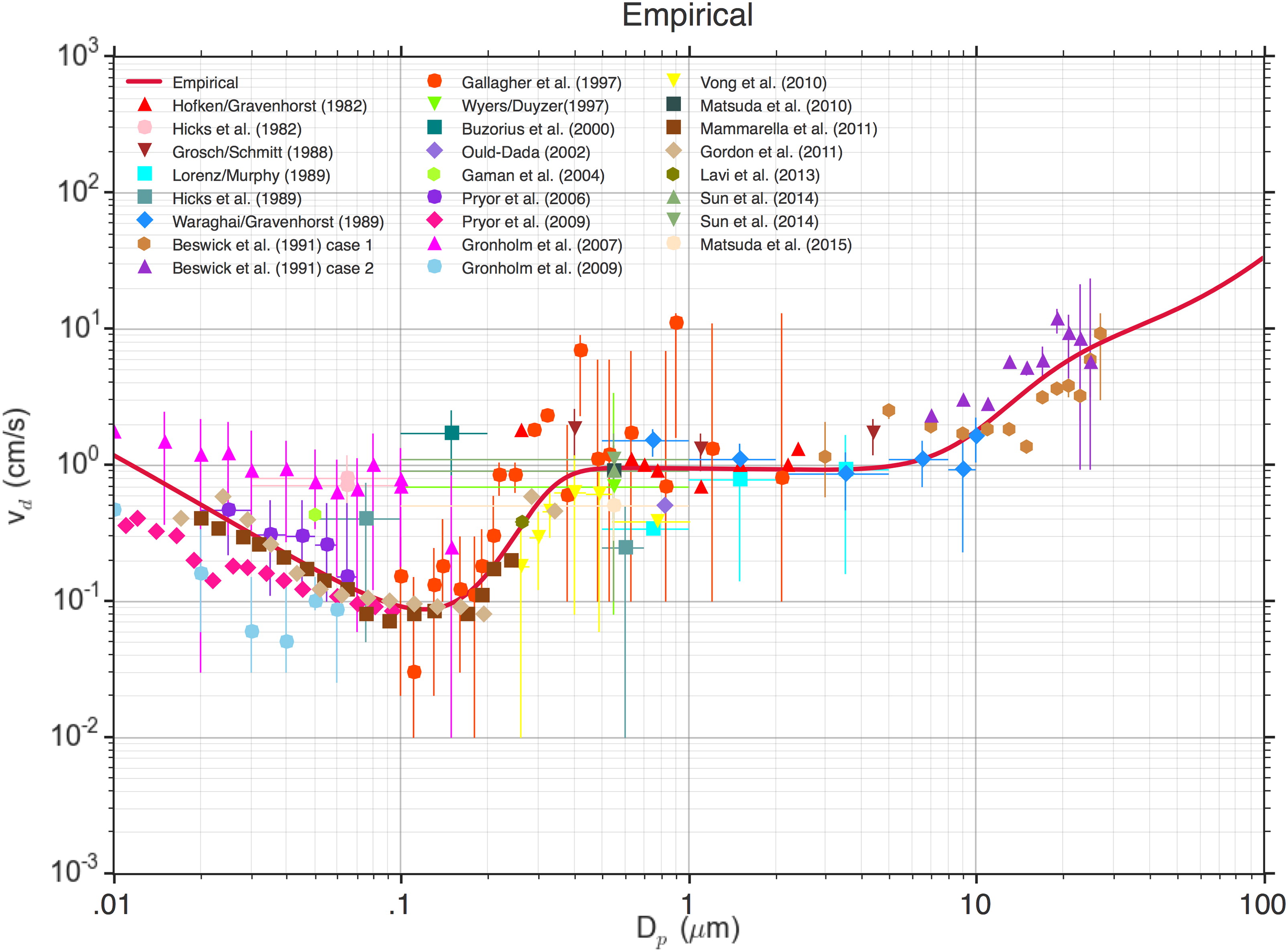
Fig. 8.
Example of the empirical representation of Vd (cm s−1) as a function of particle diameter Dp (µm), using the algorithm of Zhang et al. (2001) but including an additional efficiency for an ‘unknown’ process, thereby forcing the Vd(Dp) function to more closely represent data obtained over forests (u* = 60 cm s−1).
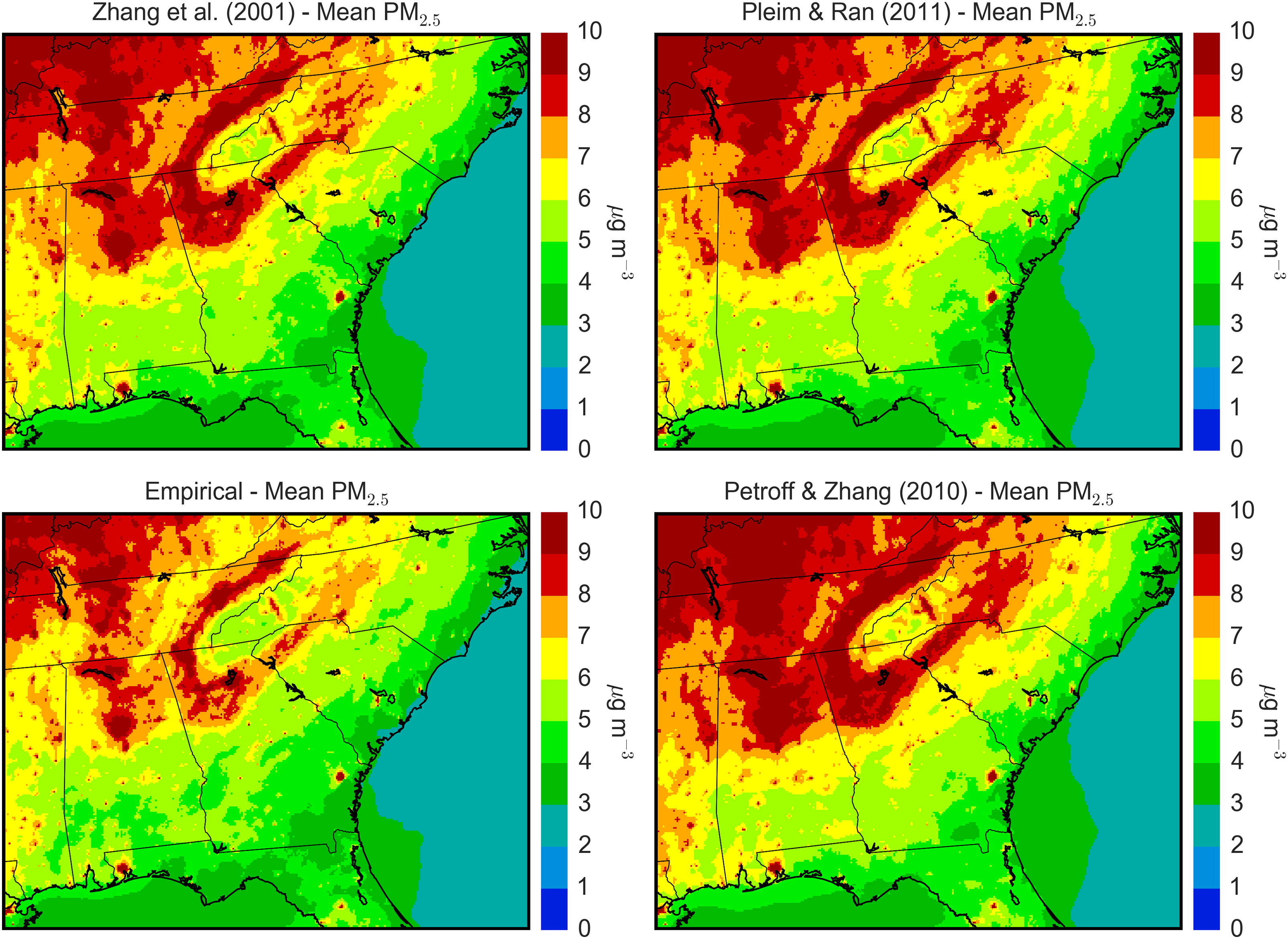
Fig. 9.
PM2.5 mean surface concentration (µg m−3) for June 14–28, 2013, with PM2.5 dry deposition algorithms of Zhang et al. (2001), Pleim and Ran (2011), Petroff and Zhang (2010), and the empirical algorithm of this work.
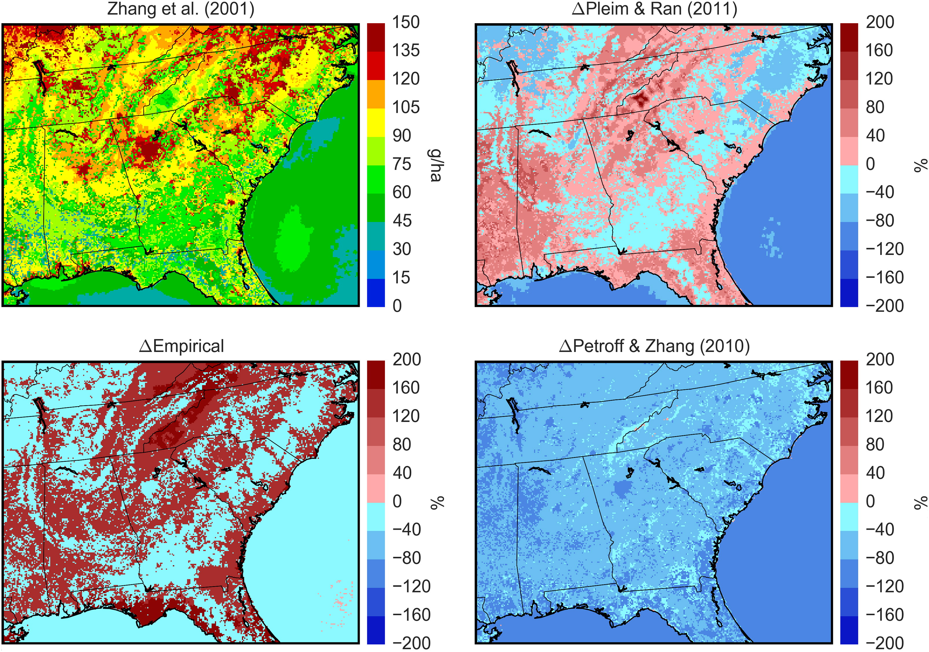
Fig. 10.
Cumulative PM2.5 dry deposition (g ha−1) (June 14–28, 2013) for the base Zhang et al. (2001) simulation and percent differences from the base for each of the tested particle deposition algorithms.
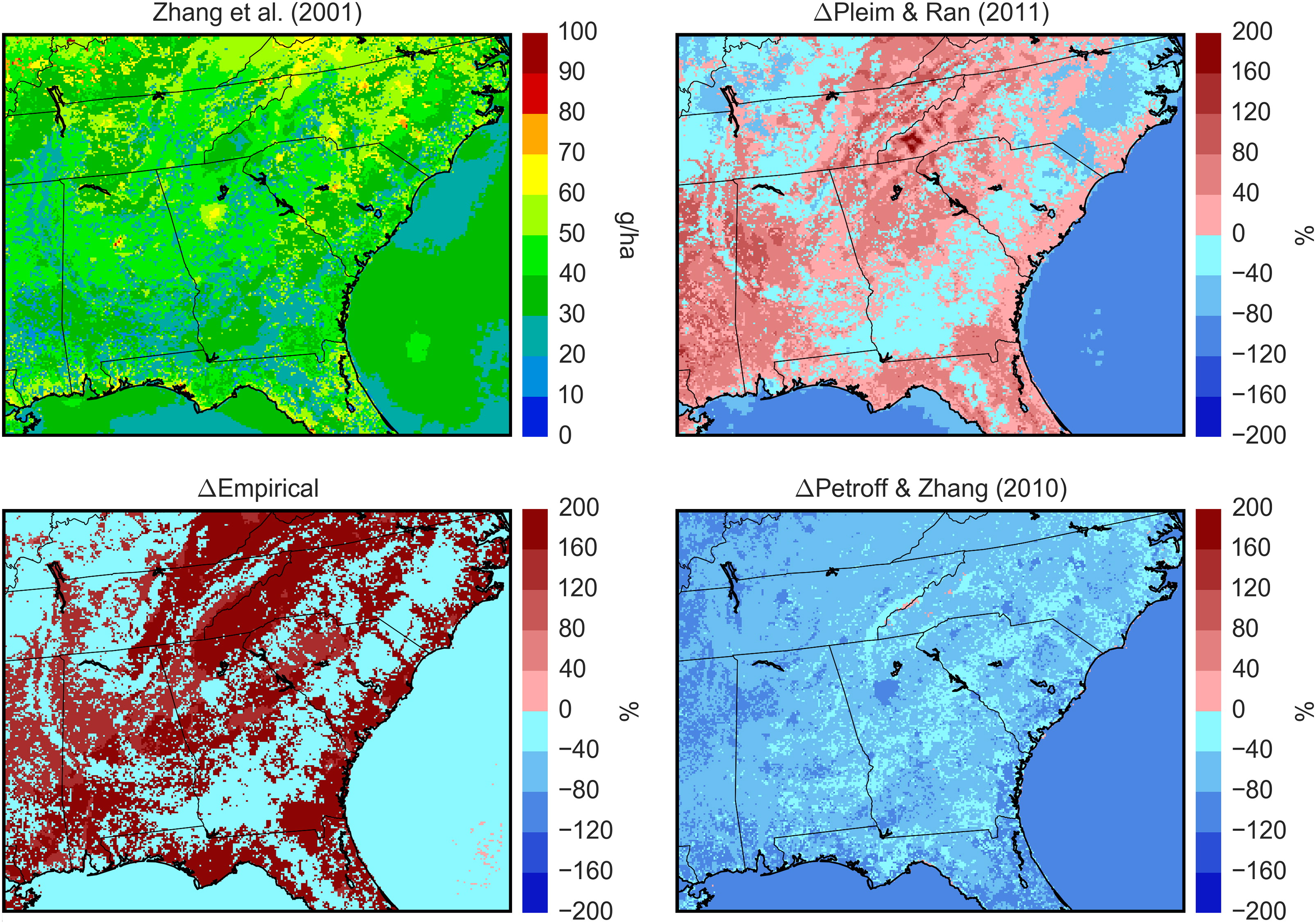
Fig. 11.
Cumulative PM2.5 SO4 2− dry deposition (g ha−1) (June 14–28, 2013) for the base Zhang et al. (2001) simulation and percent differences from the base for each of the tested particle deposition algorithms.
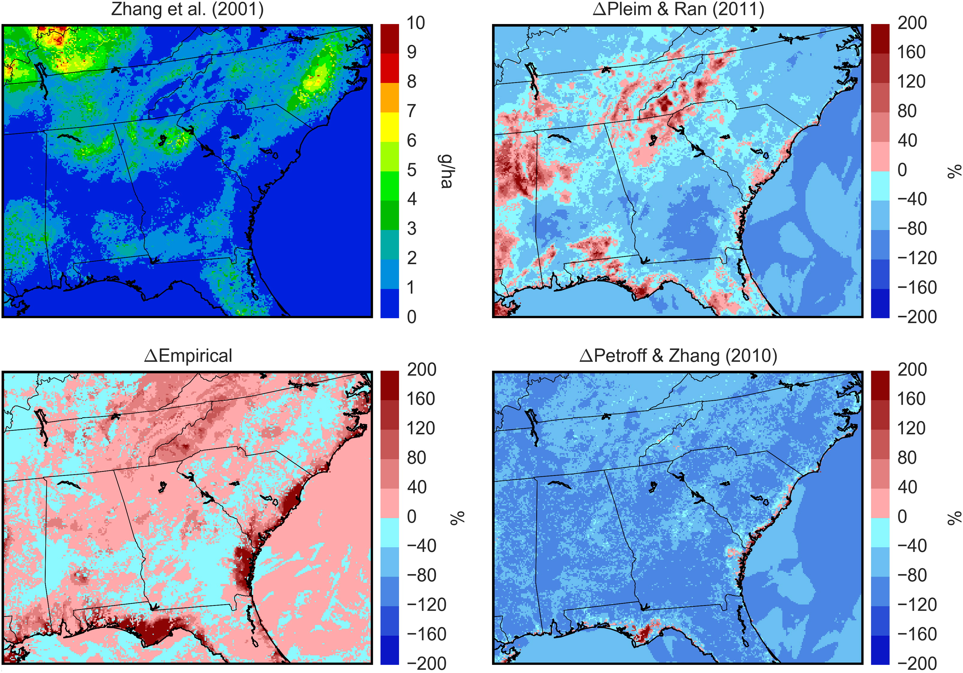
Fig. 12.
Cumulative PM2.5 NO3 − dry deposition (g ha−1) (June 14–28, 2013) for the base Zhang et al. (2001) simulation and percent differences from the base for each of the tested particle deposition algorithms.
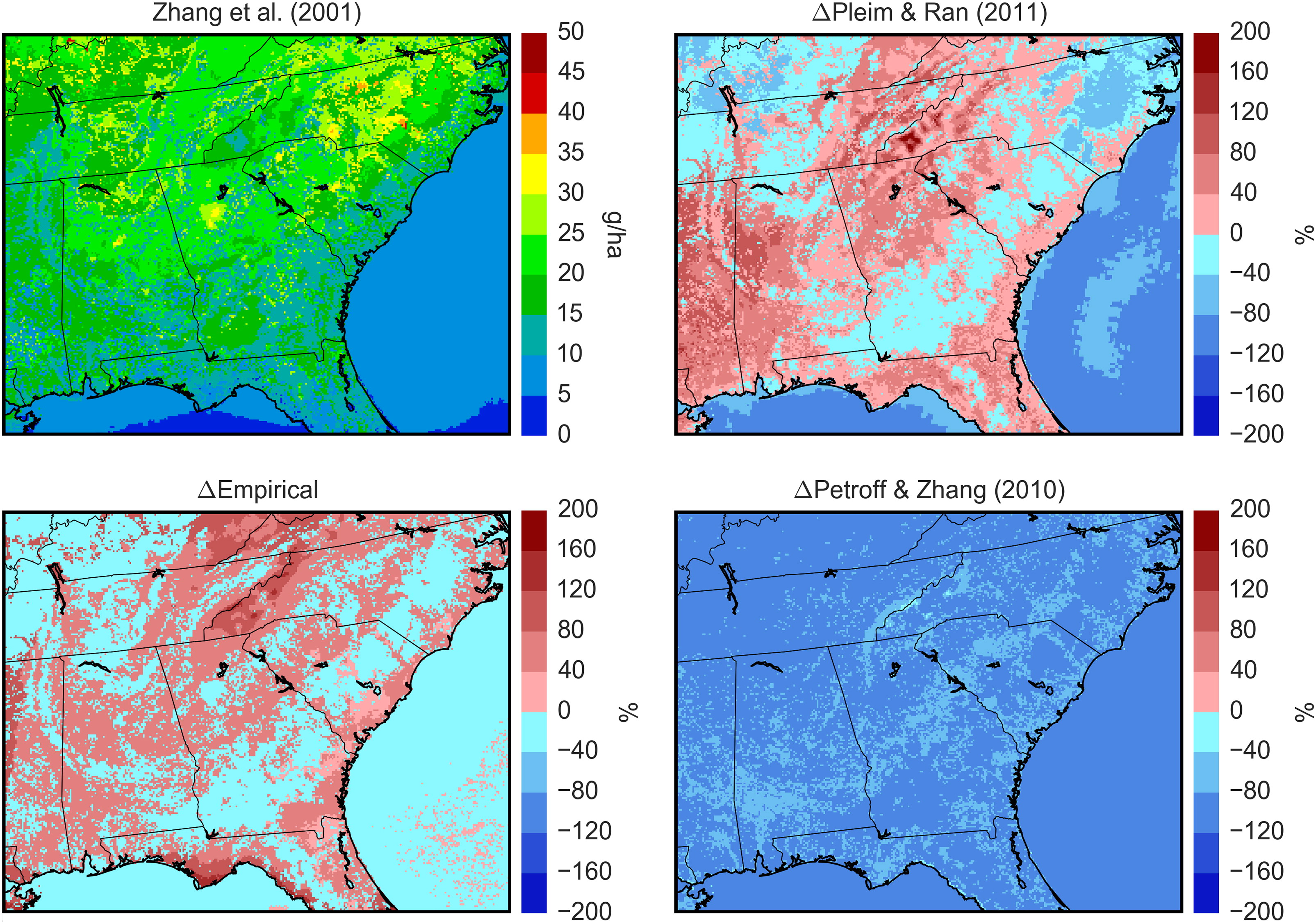
Fig. 13.
Cumulative PM2.5 NH4 + dry deposition (g ha−1) (June 14–28, 2013) for the base Zhang et al. (2001) simulation and percent differences from the base for each of the tested particle deposition algorithms.
Table 2.
Domain mean wet, dry and total PM2.5 deposition (g ha−1) for each simulation; for Wet and Dry depositions, values in parentheses are the fractions of each deposition type in the Total; for Total deposition, values in parentheses are the percentage differences in total PM2.5 deposition with respect to the base Zhang et al. simulation.
Table 3.
Mean wet, dry and total PM2.5 deposition (g ha−1) for forested grid cells only for each simulation; for Wet and Dry depositions, values in parentheses are the fractions of each deposition type in the Total; for Total deposition, values in parentheses are the percentage differences in total PM2.5 deposition with respect to the base Zhang et al. simulation.
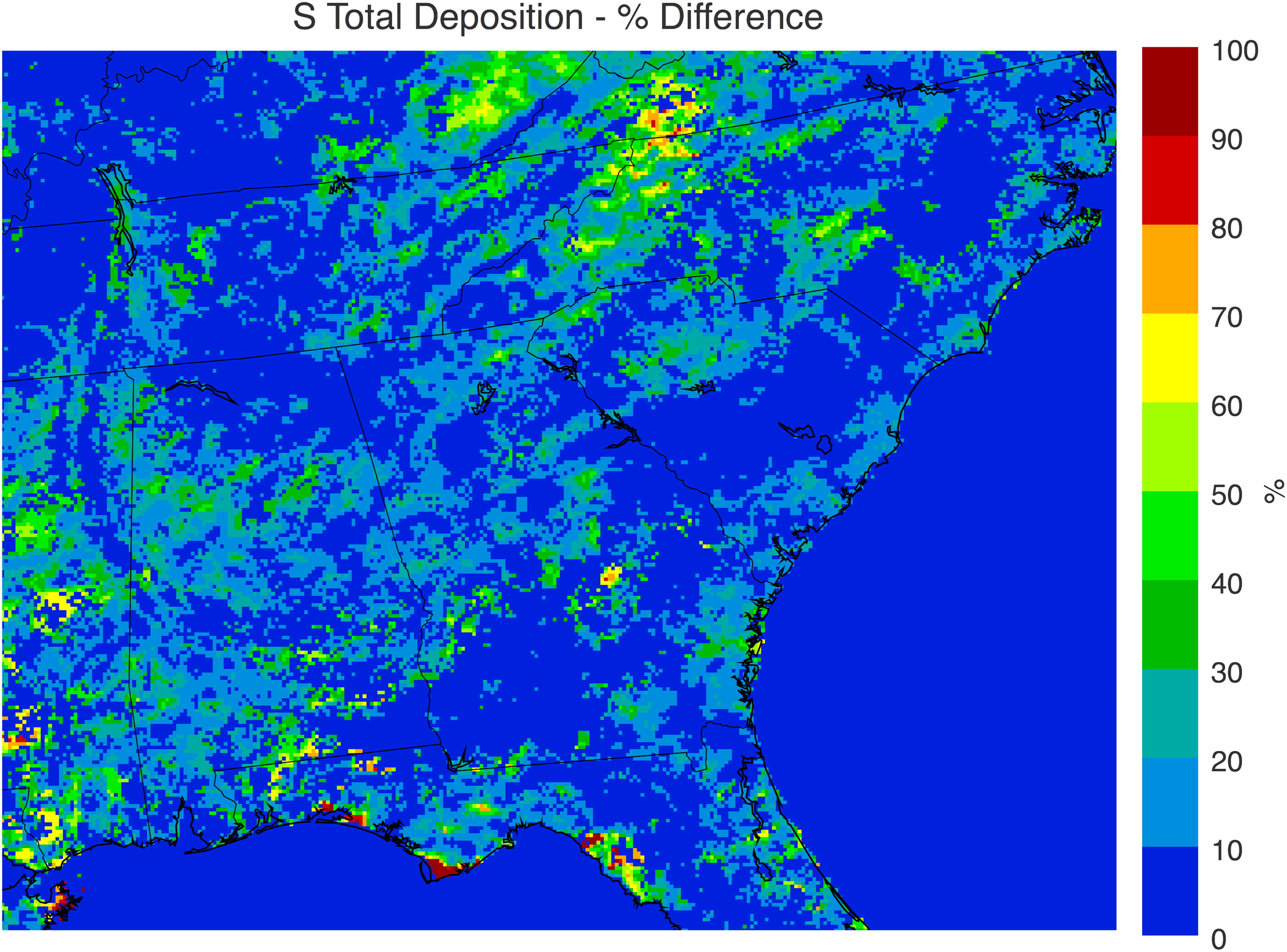
Fig. 14.
Per cent increase in total sulfur deposition (all forms of sulfur in both dry and wet deposition) between the empirical simulation and the base Zhang et al. simulation. Maximum increase = 160.6%; Domain mean increase = 7.5%.
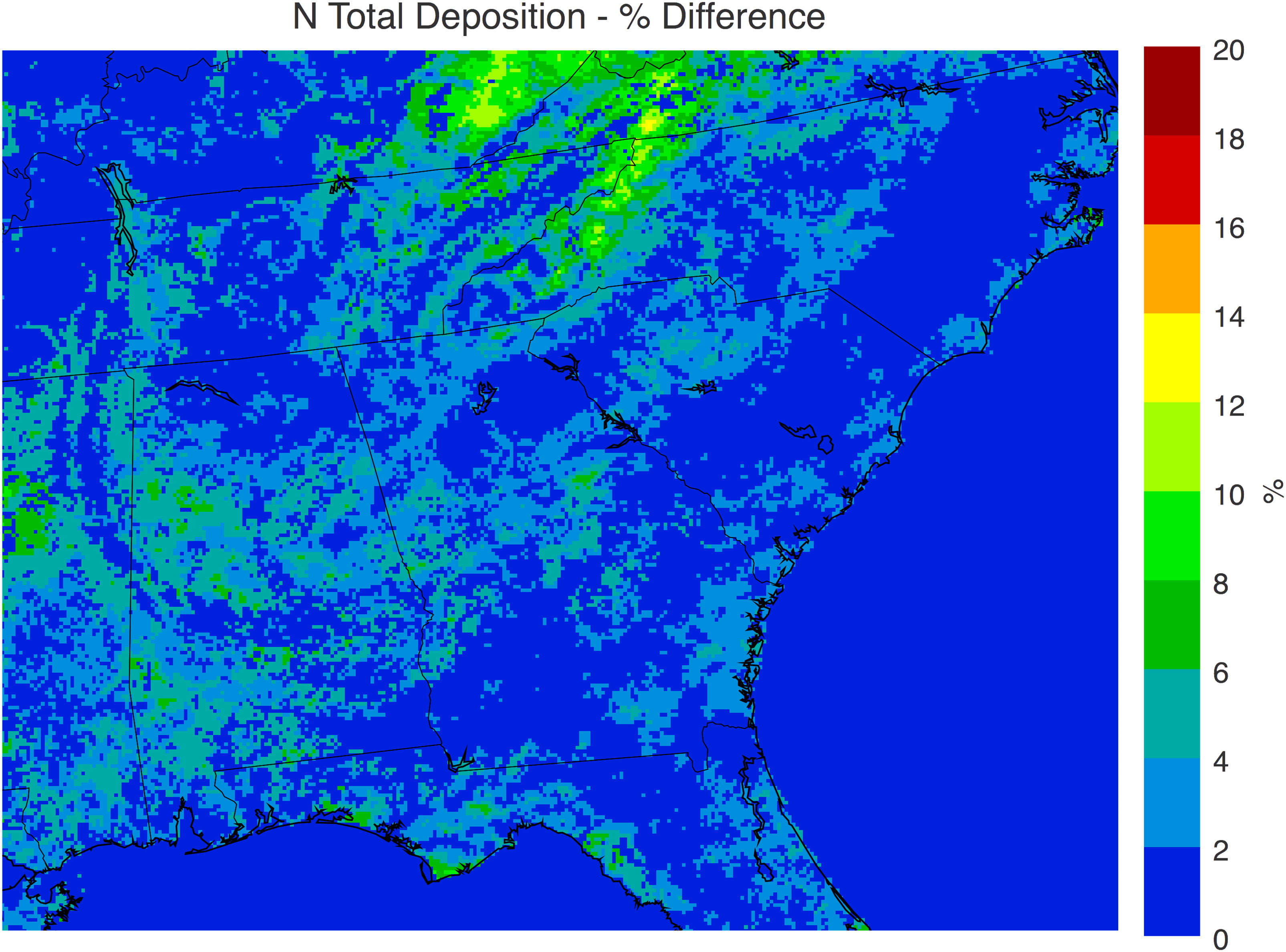
Fig. 15.
Percent increase in total nitrogen deposition (all forms of nitrogen in both dry and wet deposition) between the empirical simulation and the base Zhang et al. simulation. Maximum increase = 13.0%; Domain mean increase = 1.3%.
Table 4.
Mean bias (g ha−1) and normalised mean bias (%) for model simulation vs CASTNet estimated PM2.5 species dry deposition from filter samples obtained June 18–25, 2013 (N = 15). Model depositions accumulated to correspond to the CASTNet filter samples over the one-week time period (https://www.epa.gov/castnet).
Table 5.
Mean bias (µg m−3) and normalised mean bias (%) for model simulation vs CASTNet PM2.5 species concentrations from filter samples obtained June 18–25, 2013 (N = 15). Model concentrations averaged to correspond to the CASTNet filter samples over the 1-week time period (https://www.epa.gov/castnet).