
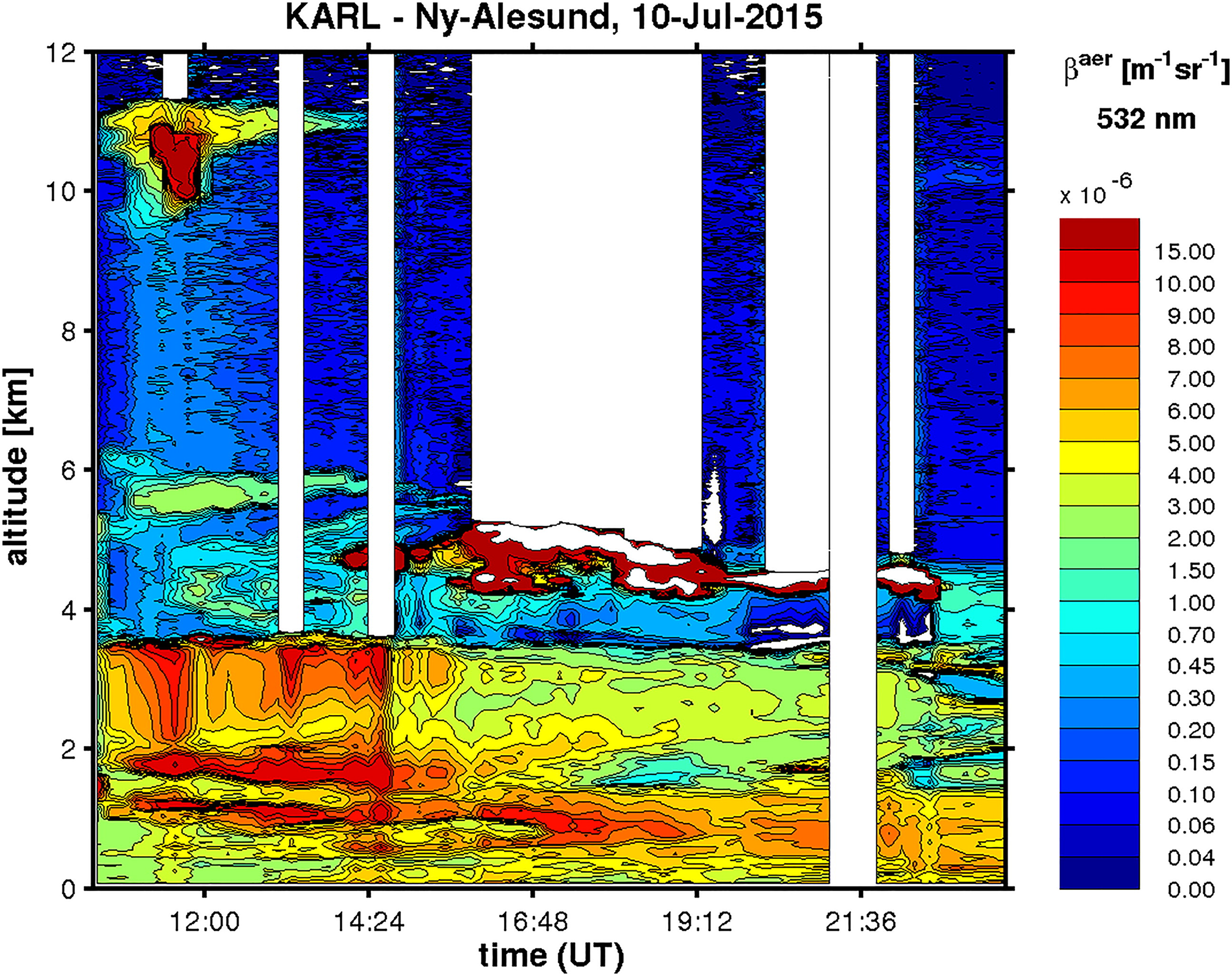
Fig. 1.
Aerosol backscatter coefficient on 10 July 2015 as recorded by the KARL lidar at 532 nm (colour-coded). White stripes indicate excluded data due to multiple scattering.
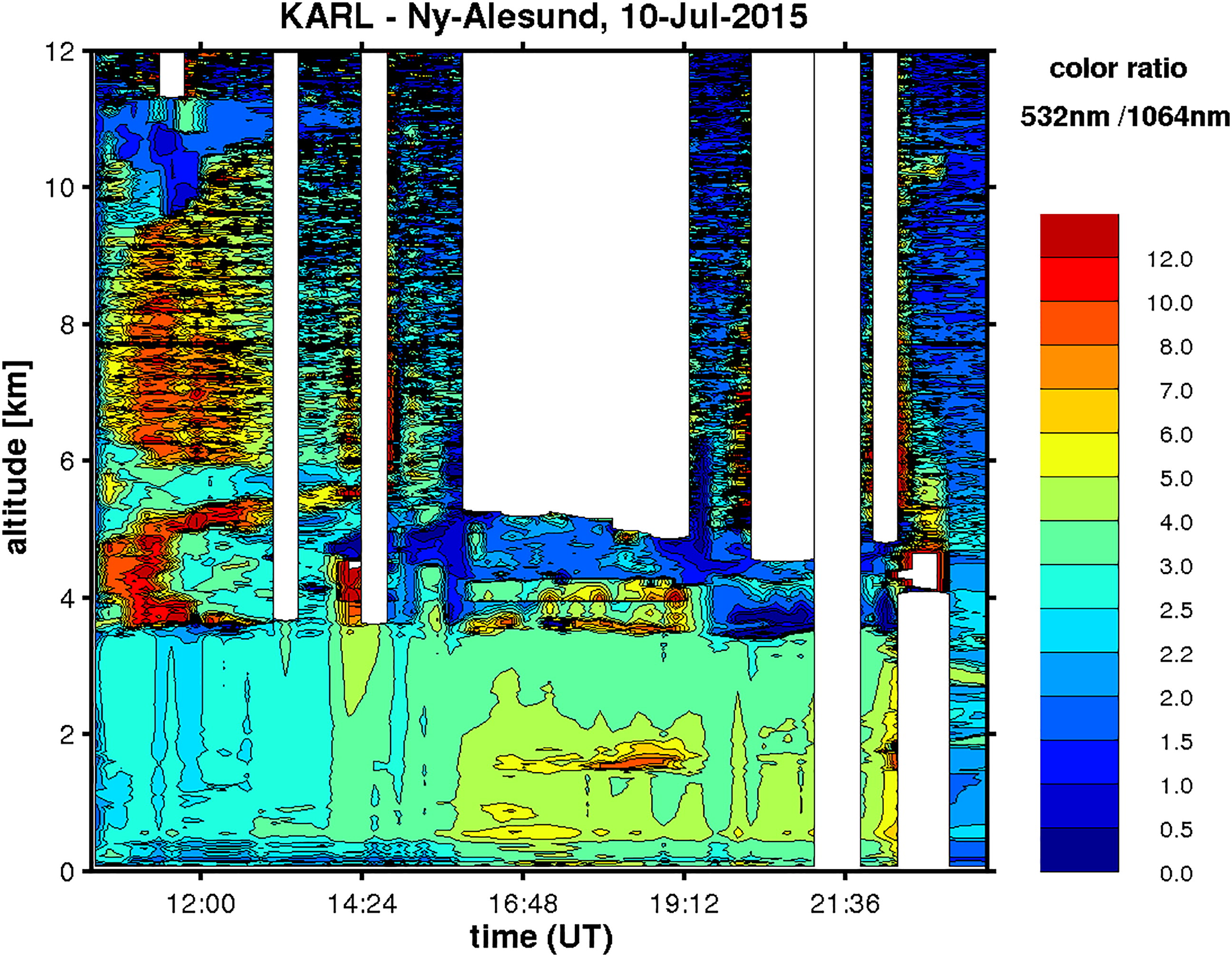
Fig. 2.
Colour ratio derived from the wavelengths of 532 nm and 1064 nm as a rough indicator of the particles’ size.
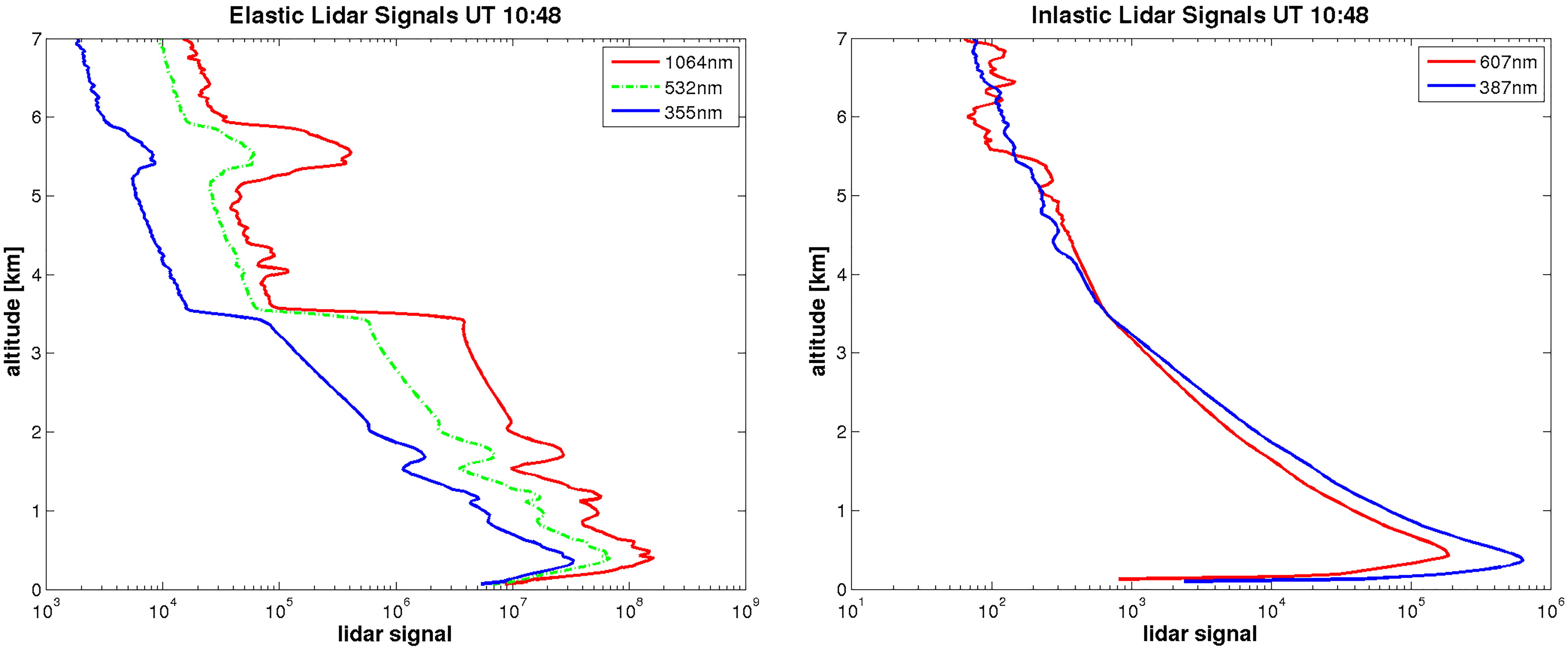
Fig. 3.
Exemplary lidar profiles in for the elastic (left) and inelastic scattering (right) for the time UT 11:48, contemporary to the radiosonde.
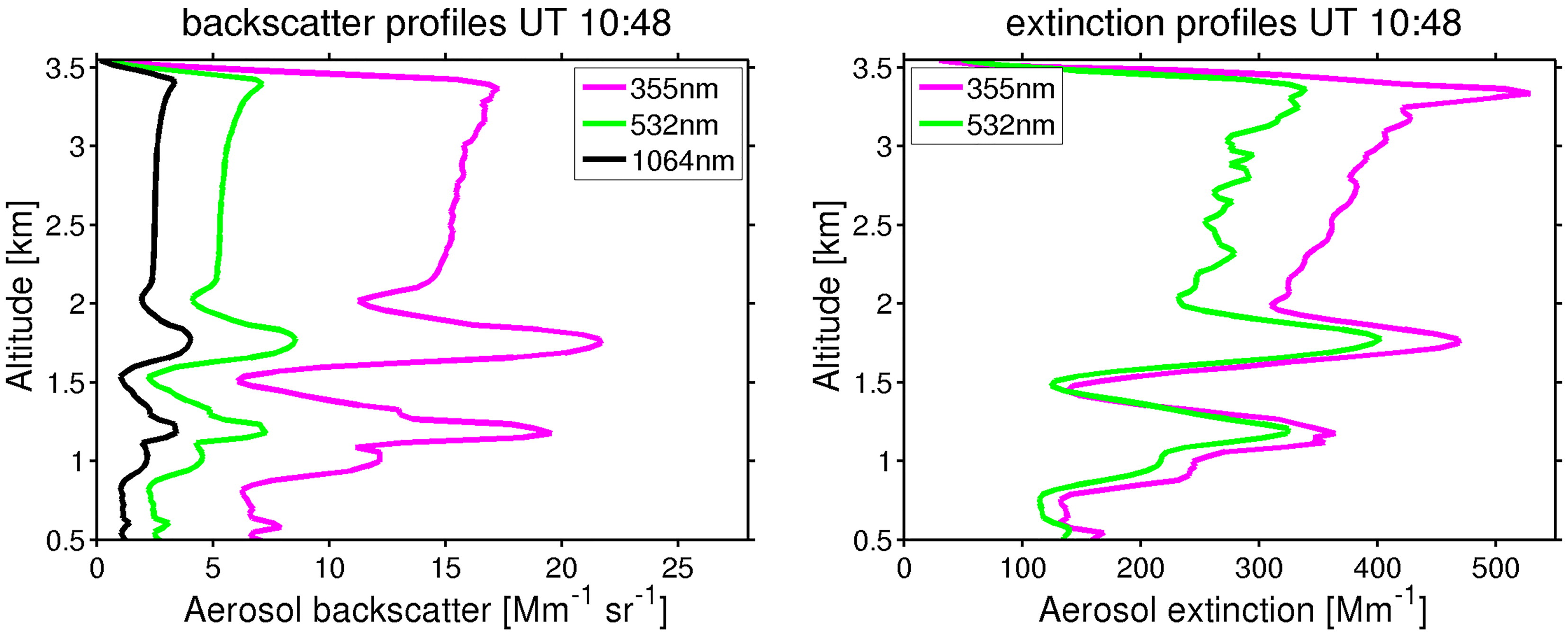
Fig. 4.
Profiles of the aerosol backscatter coefficient (left) and the aerosol extinction coefficient (right) for the time of the launch of the radiosonde.
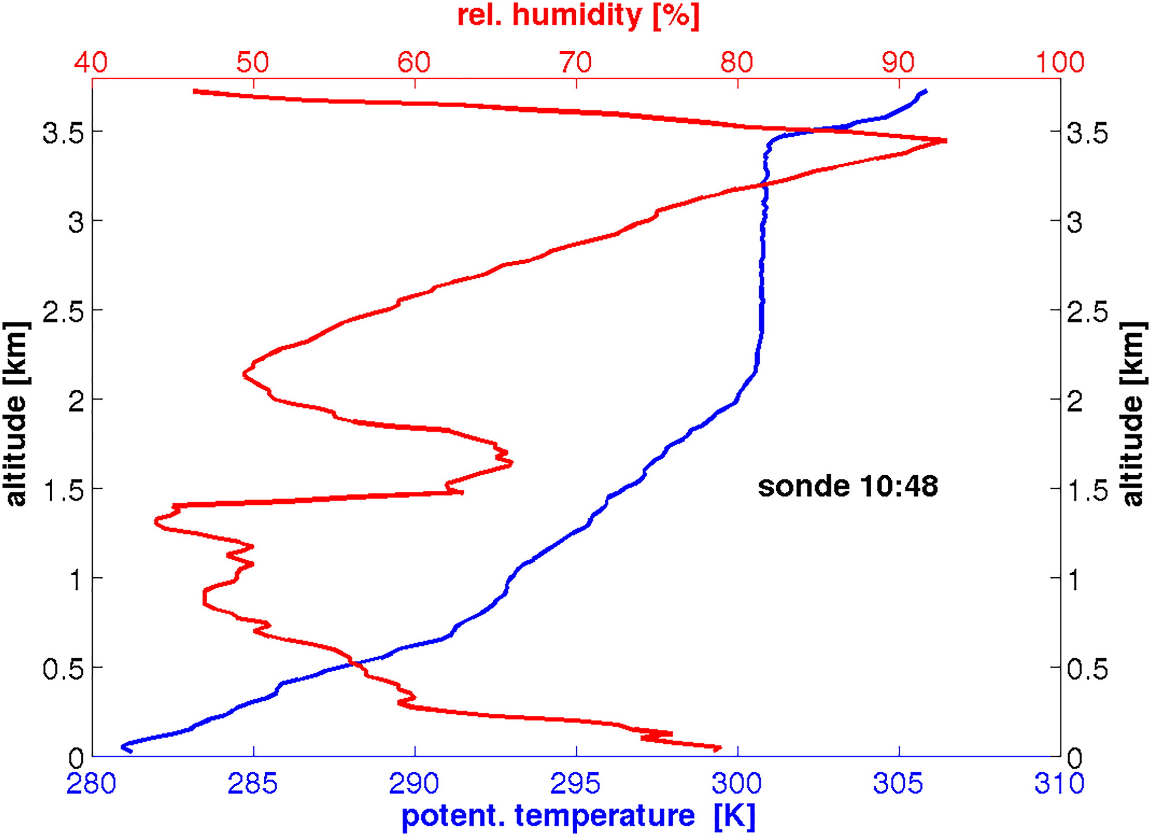
Fig. 5.
Radiosonde profiles on 10 July 2015 of potential temperature (blue) and relative humidity over water (red) from a RS-92 sonde on 10 July, 2015.
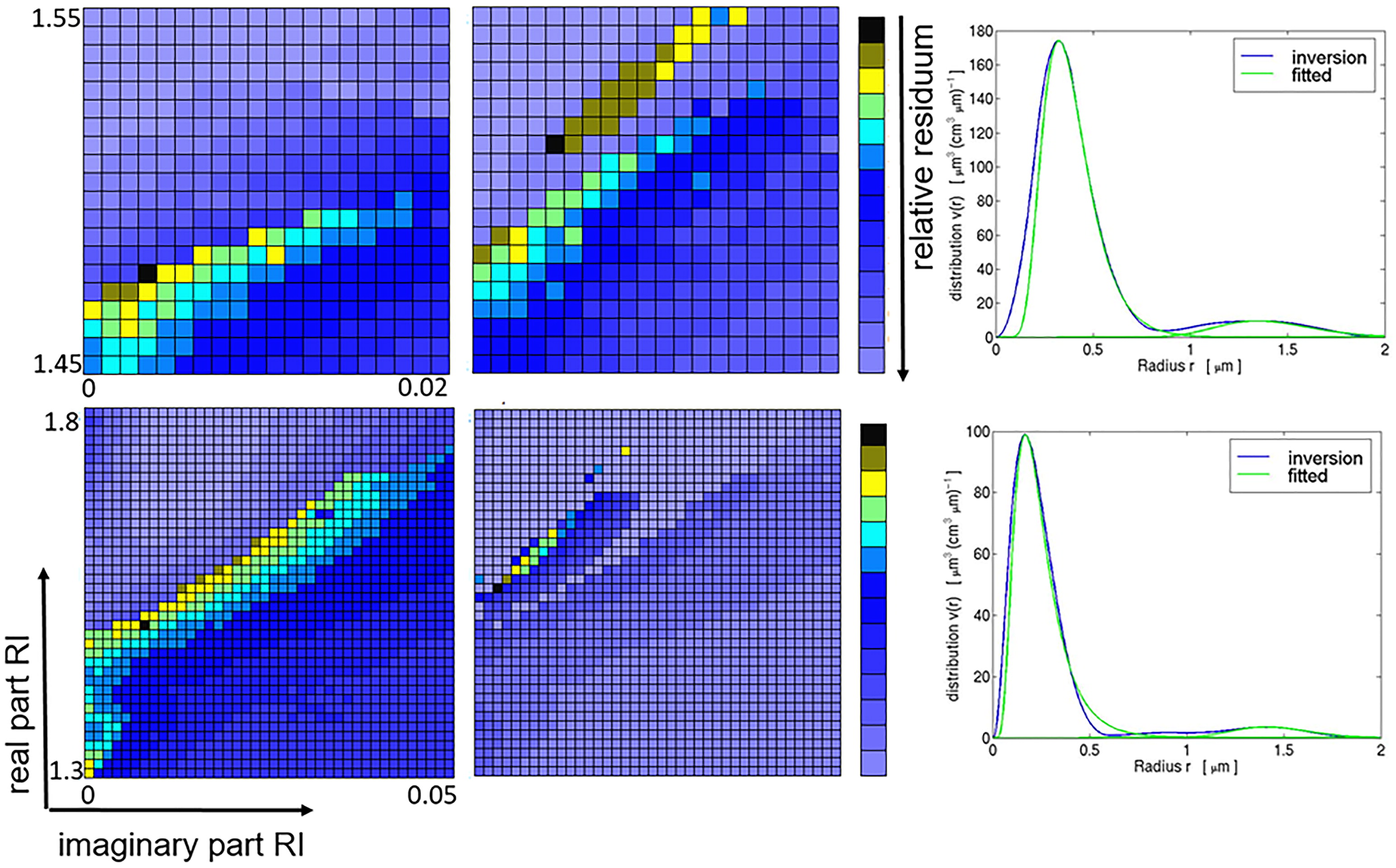
Fig. 6.
First row: Inversion results for layer 2 (1717–1777 m). Left, centre, right: (20 × 20)-grid of refractive index RI at 10:48 UTC, (20 × 20)-grid of RI at 12:07 UTC, retrieved volume distribution at 10:48 UTC. Second row: Inversion results for layer 3 (2166–2436 m). Left, centre, right: (40 × 40)-grid of RI at 10:48 UTC, (40 × 40)-grid of RI at 12:07 UTC, retrieved volume distribution at 12:07 UTC.
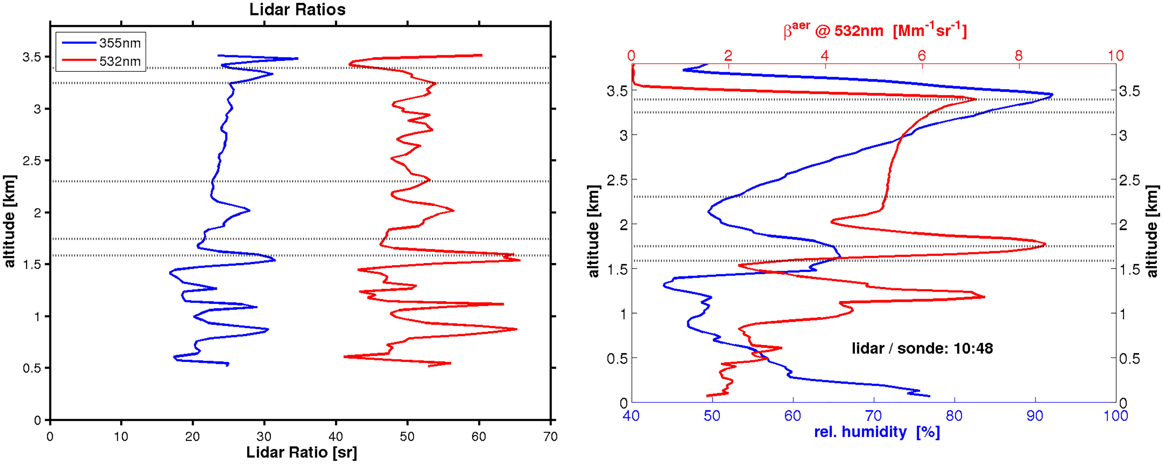
Fig. 7.
Selection of the layers (vertical dotted lines) in terms of the lidar ratios (left), RH and aerosol backscatter coefficient (right) (Data for 10:48 UTC).
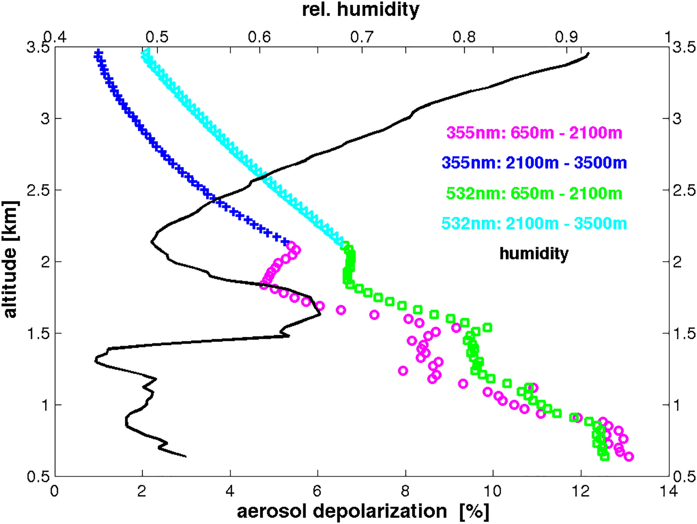
Fig. 8.
Aerosol depolarisation at 355 nm and 532 nm and relative humidity (black line) for comparison.
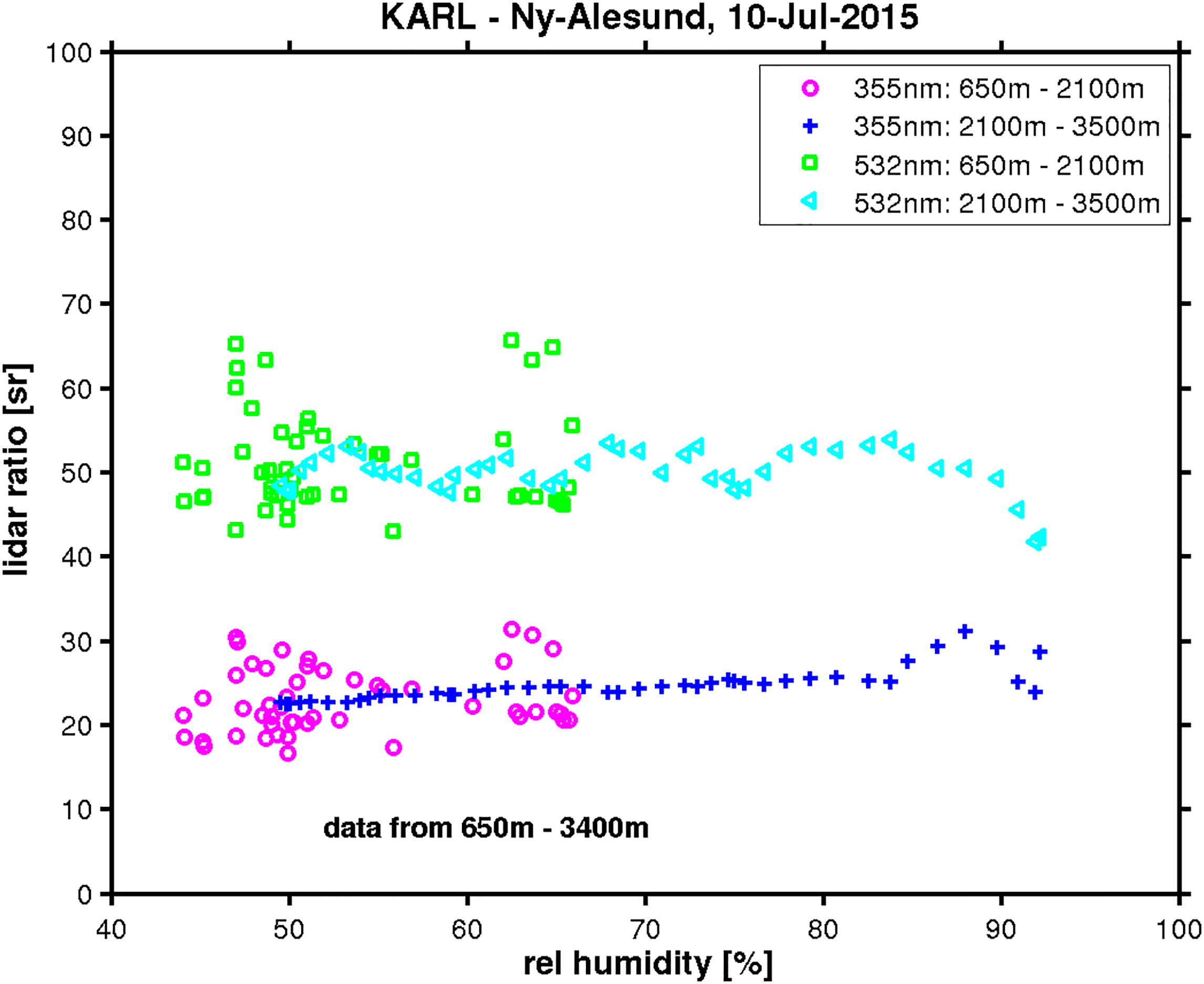
Fig. 9.
The lidar ratio as function of the relative humidity for lidar data contemporary to the radiosonde (10:48 – 10:59 UTC).
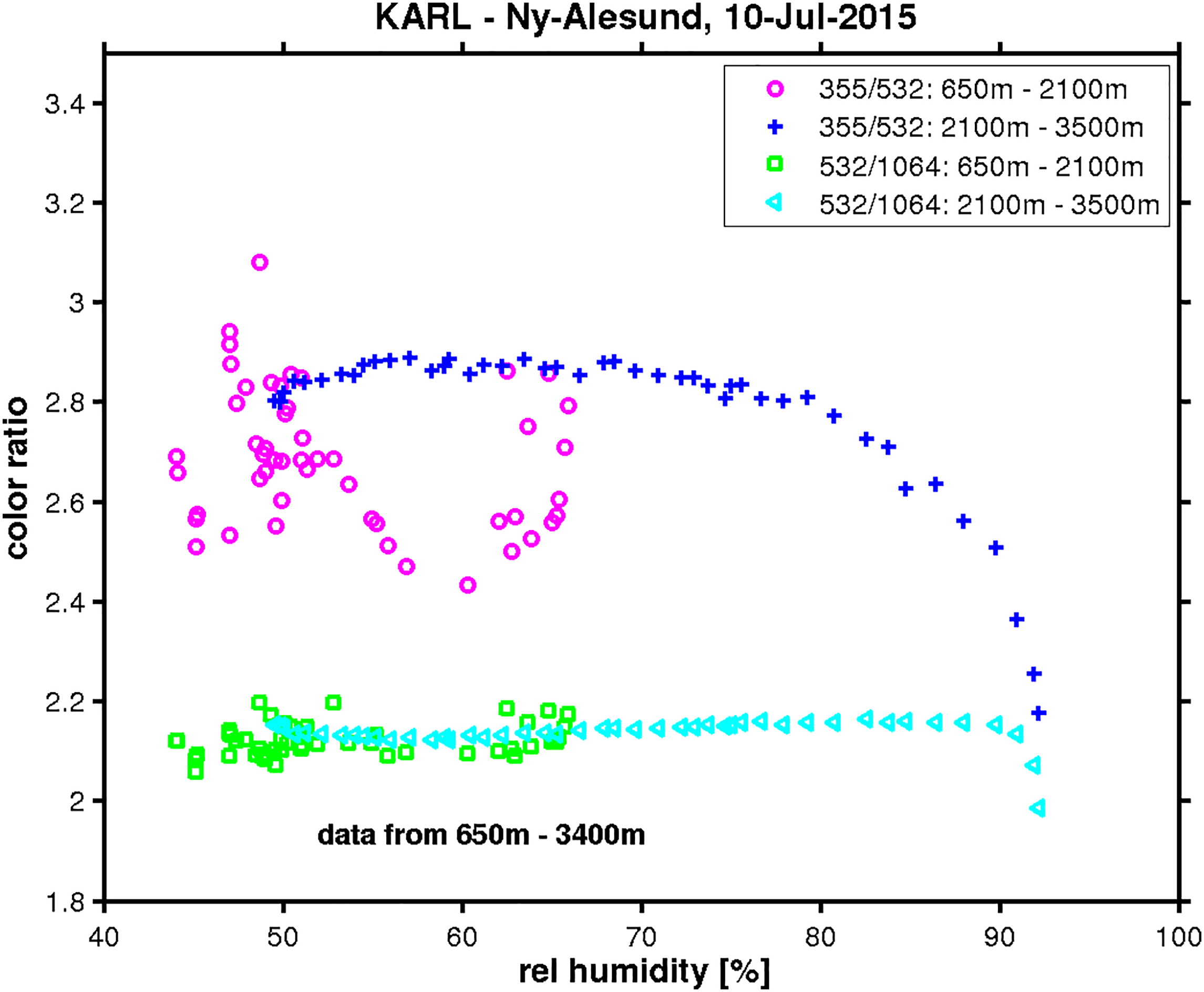
Fig. 10.
Colour ratios in 355/532 and 532/1064 as function of the relative humidity for lidar data contemporaneous to the radiosonde.
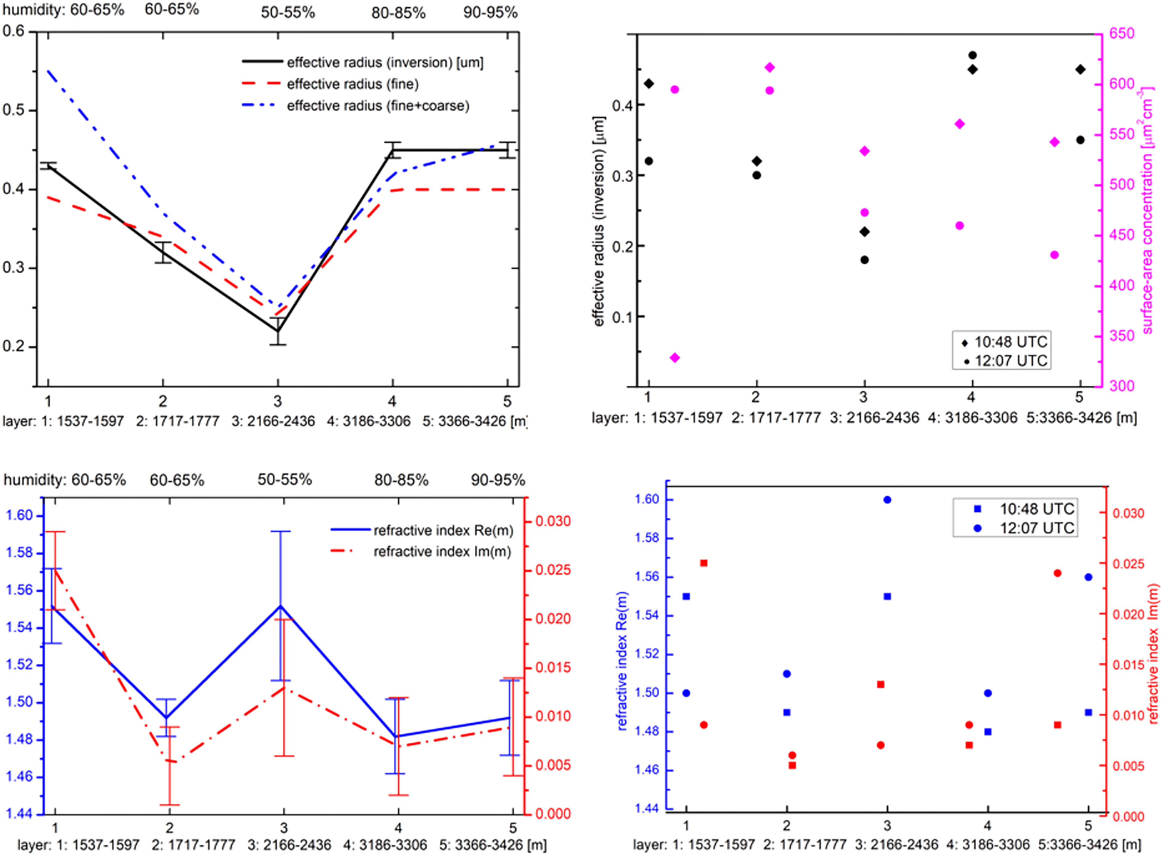
Fig. 11.
First row: Comparison of effective radii. Left: Effective radii (fine, fine+coarse and complete inverted) for the five investigated layers with different relative humidity at 10:48 UTC, showing the hygroscopic growth. Right: Comparison of the inverted effective radius and surface-area concentration for the five layers at two different times: 10:48 UTC and 12:07 UTC, showing the stability of the parameters. Second row: Comparison of the real and imaginary part of the refractive index. The error bar represent the standard deviation from the mean value.
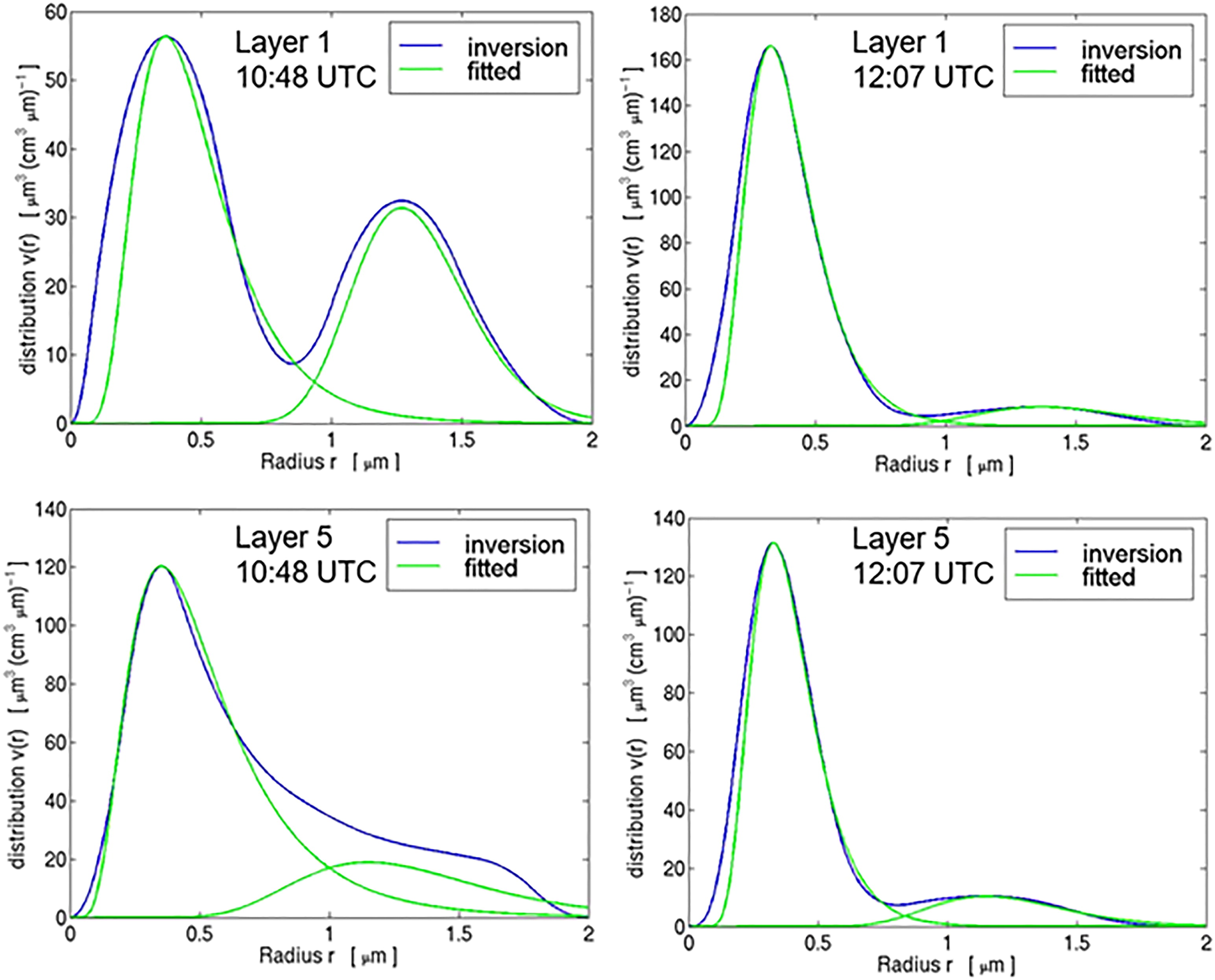
Fig. 12.
Retrieved volume distribution and log-normal fits for fine and coarse mode.
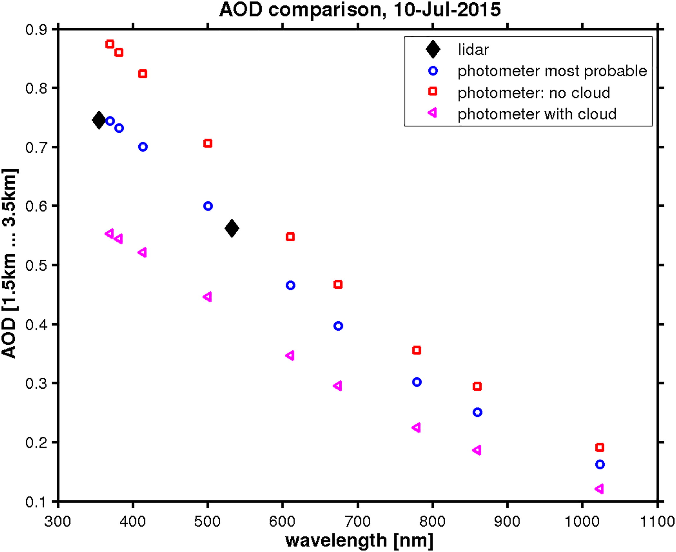
Fig. 13.
Integrated aerosol extinction in a layer [1500 m …. 3500 m] from the lidar (black diamonds) and photometer AOD for that interval for different assumptions on cloud contamination.
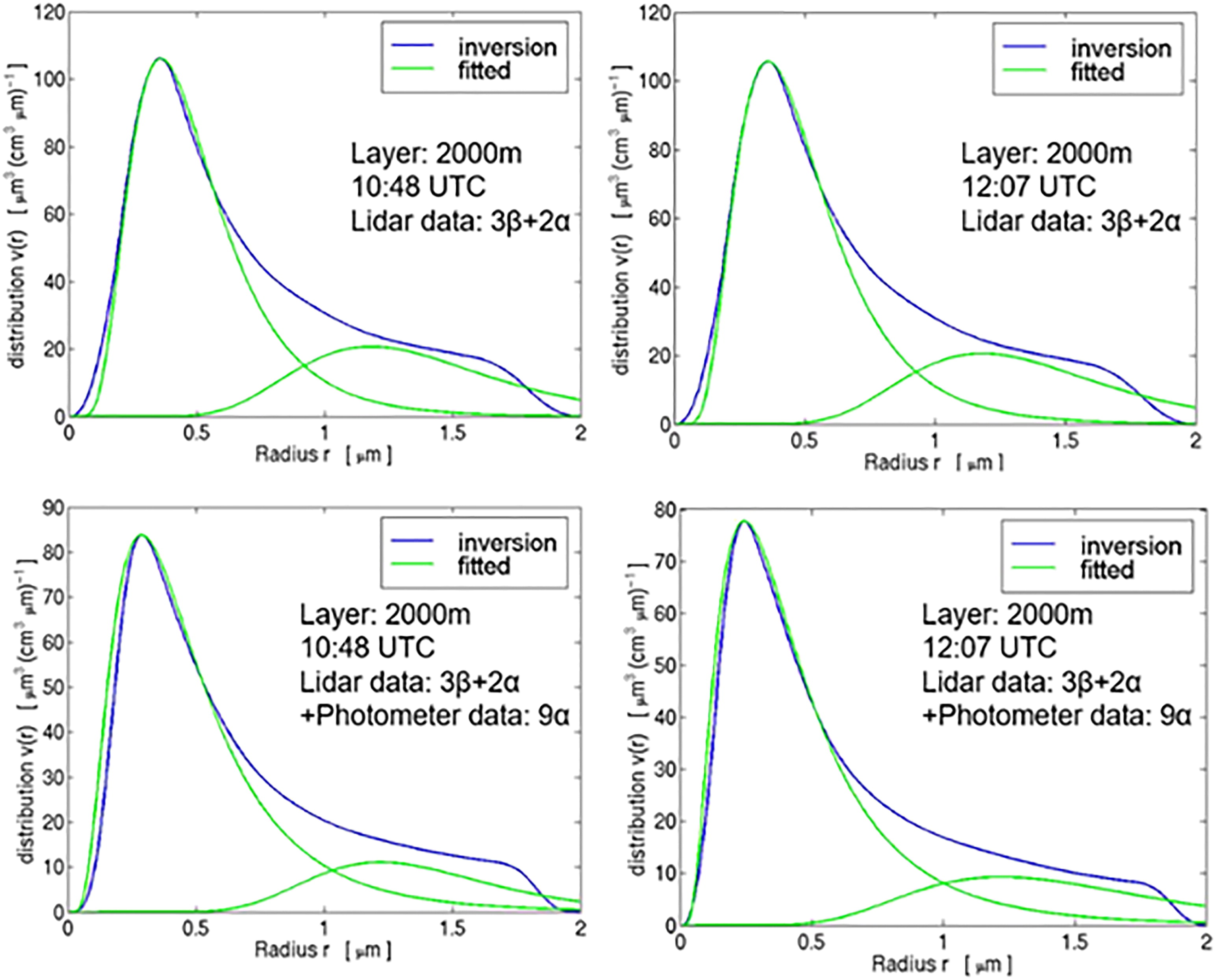
Fig. 14.
Size distribution for the whole evaluable layer from 1500 m to 3500 m altitude, above: only lidar (3 backscatter and two extinction coefficients), below: lidar and photometer, hence in total same 3 backscatter and 2 + 9 extinction coefficients.
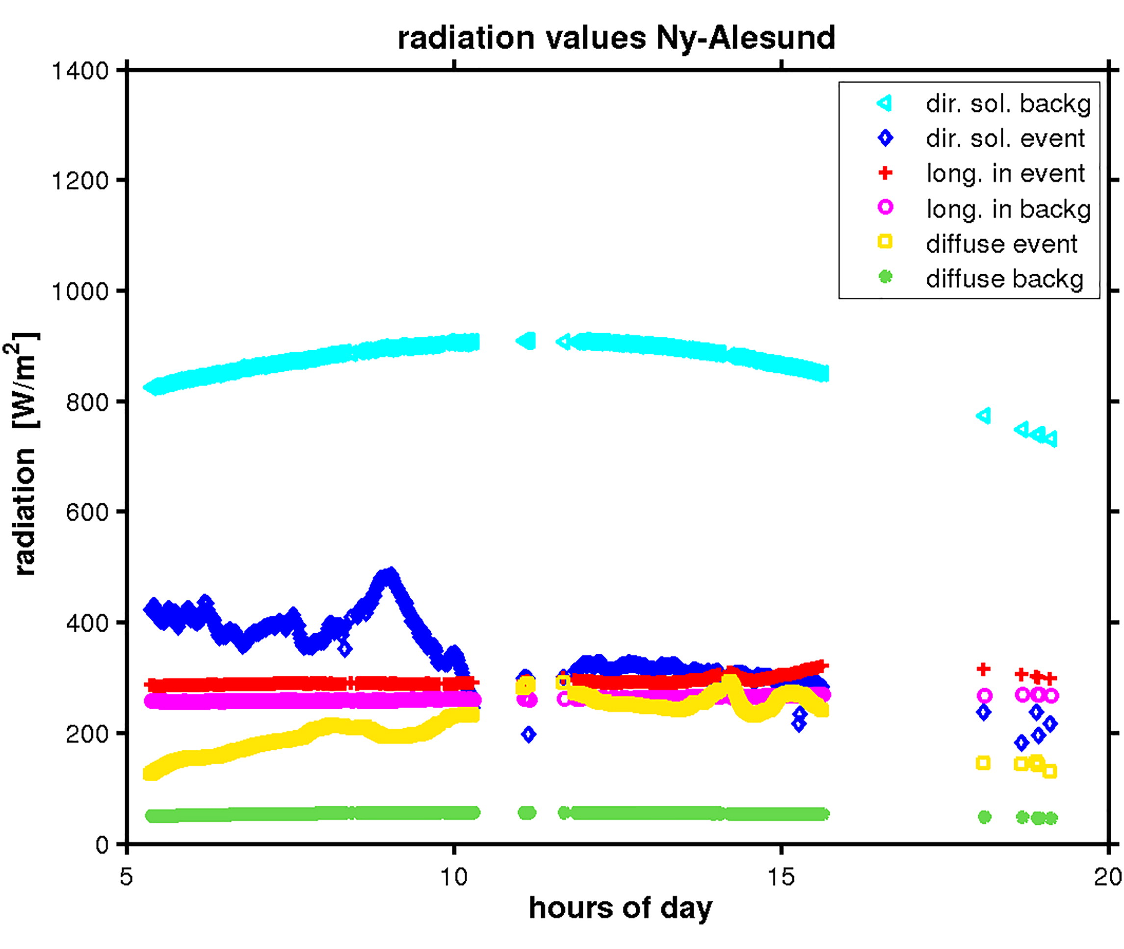
Fig. 15.
Comparison between (incoming) radiation components: direct and diffuse solar and longwave downward radiation for the BB event (10 July, 2015) and a clear background day (10 July, 2016).
Table 1.
This table collects all microphysical properties for the first measurement time at 10:48 UTC.
Table 2.
This Table collects all microphysical properties for the second measurement time at 12:07UTC.
[i] Remark: [fine/coarse] is only valid for columns 4–8. The values v t and a t refer to the inverted total distribution (the blue curves in Figures 12 and 14, not to the sum of the log-normal fits).
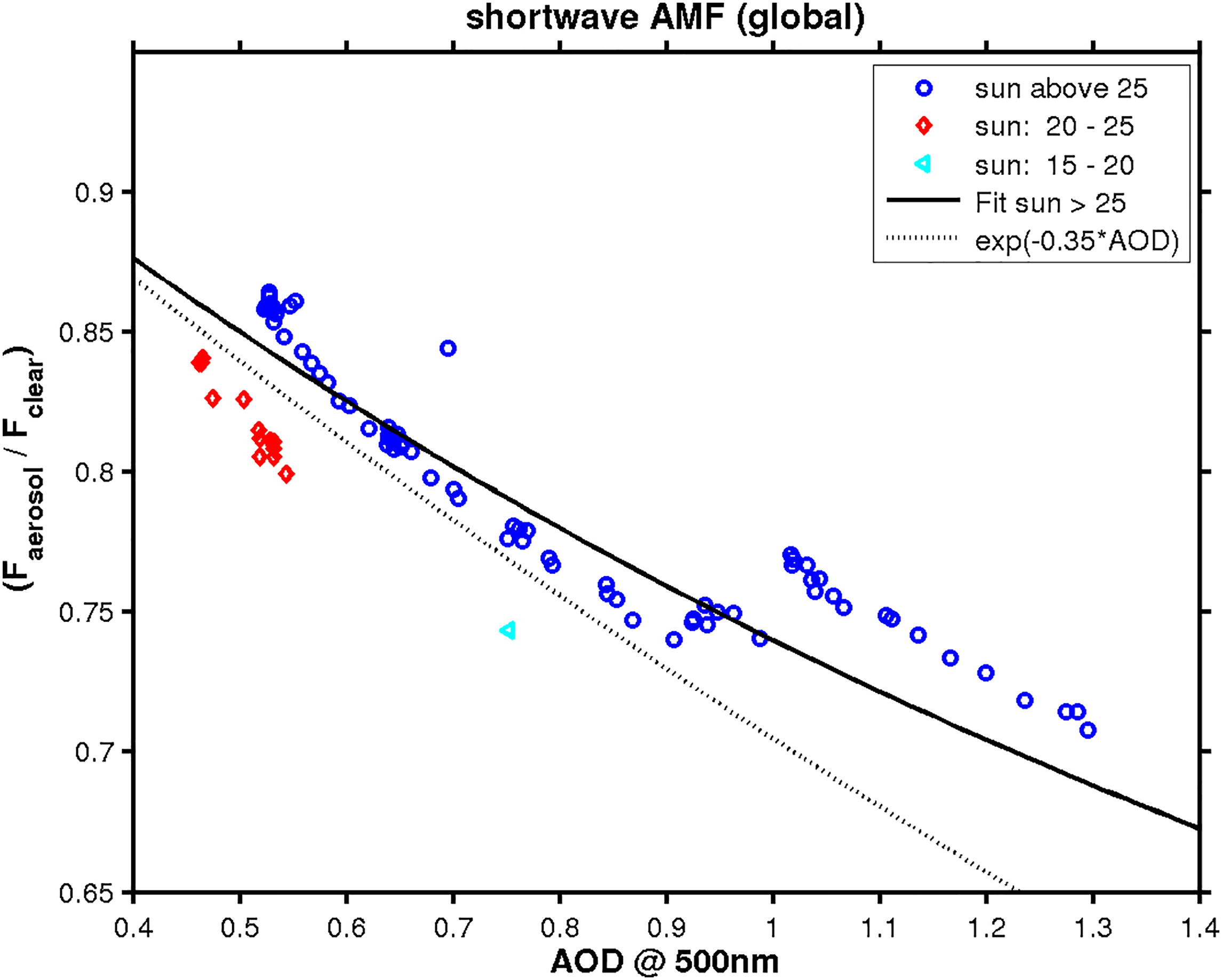
Fig. 16.
Aerosol modification factor for shortwave (global) radiation as a function of AOD.
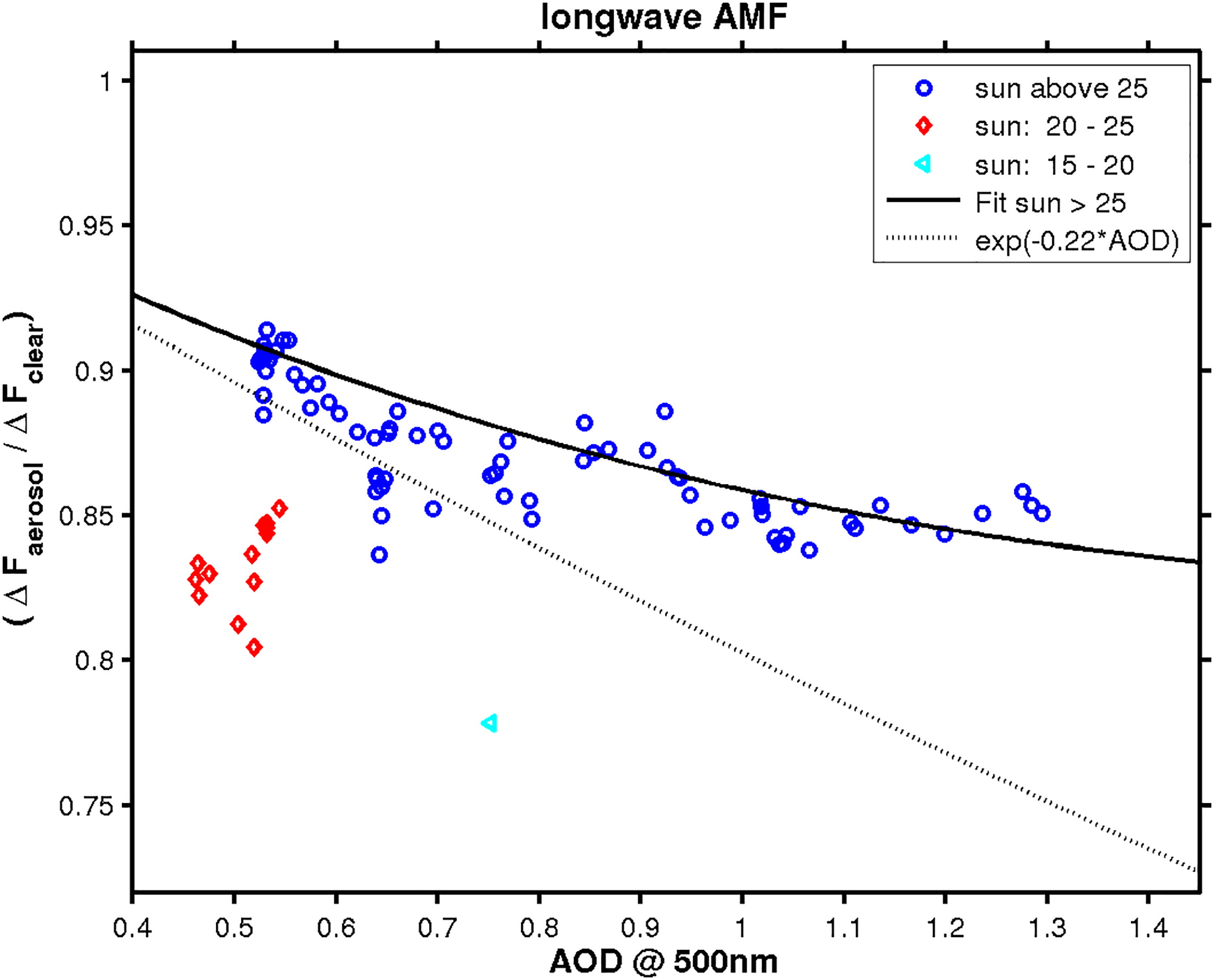
Fig. 17.
Aerosol modification factor for longwave (global) radiation as a function of AOD.
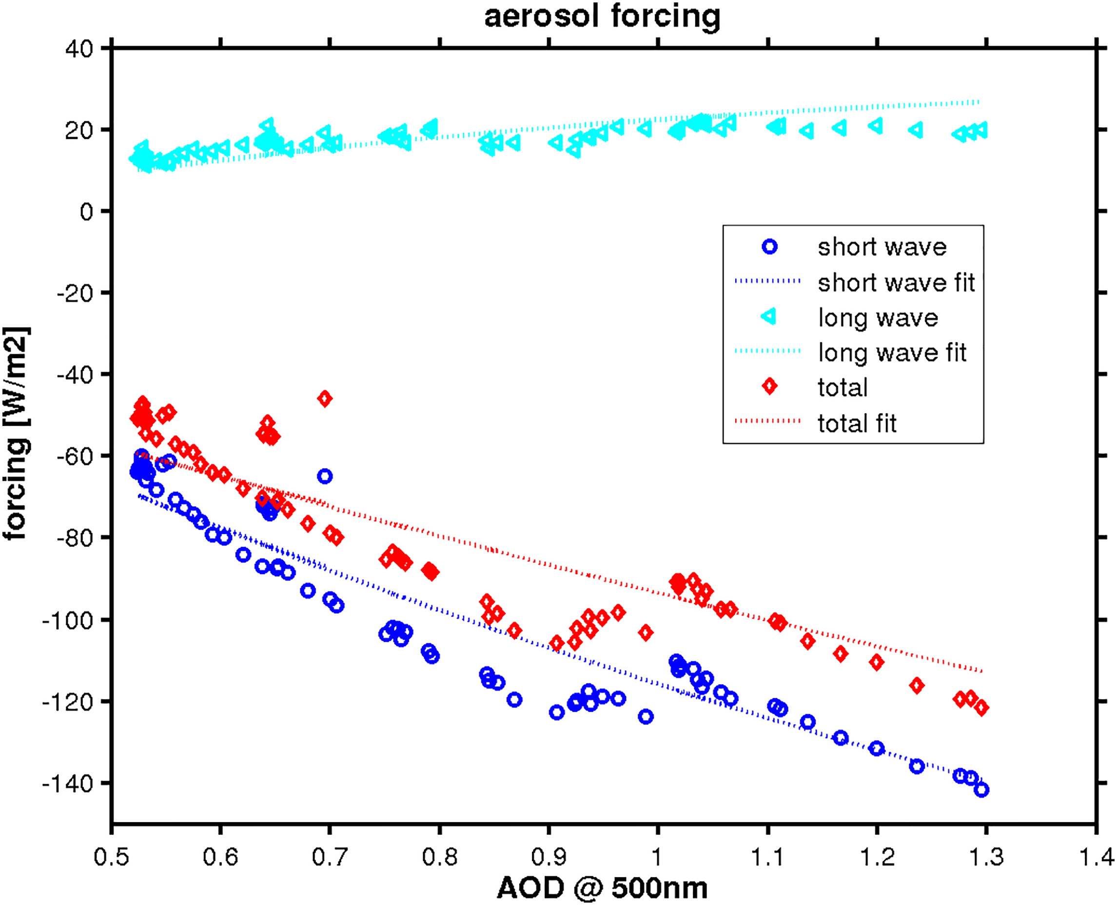
Fig. 18.
Aerosol forcing as a function of AOD.