
Fig. 1.
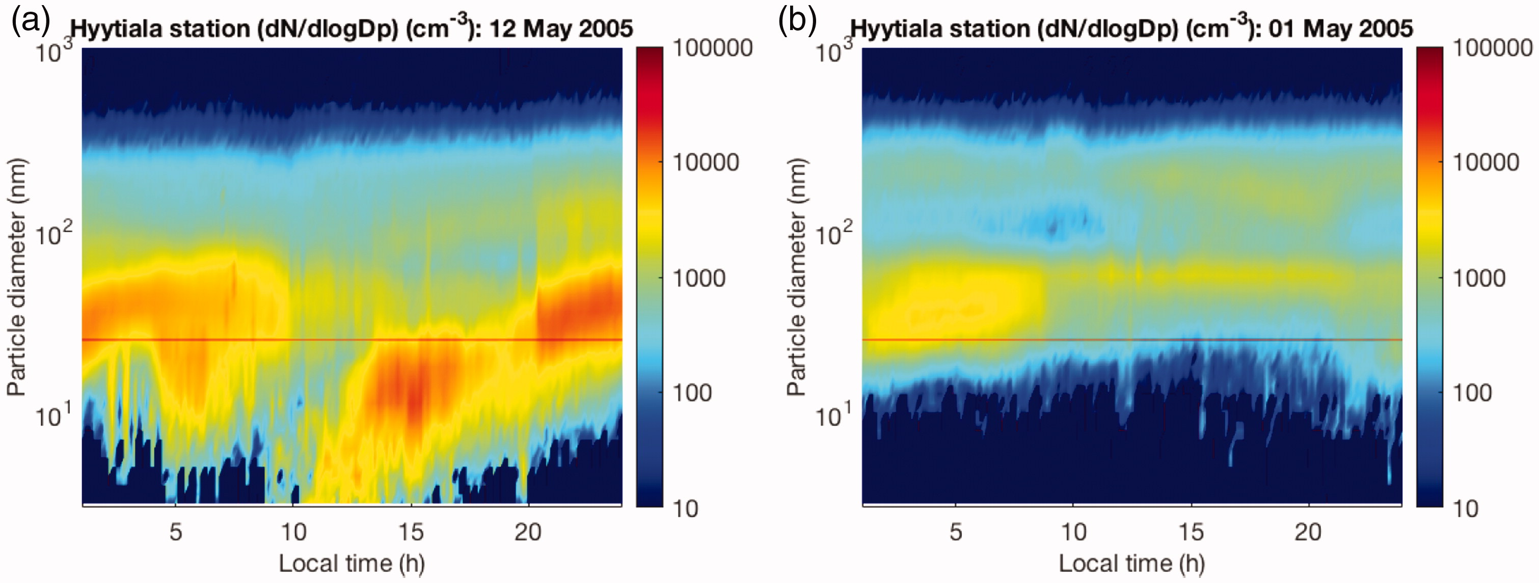
Examples of an event (a) and a non-event (b) day at Hyytiälä, Finland, in May 2005. The x-axis shows one 24-h time period whereas the y-axis shows the range of particle size diameters (from 3 to 1000 nm). The color scale indicates particle concentration (cm– 3). In (a) one can clearly see aerosol particles forming around noon and then growing into larger sizes. This data was accessed via Smart-SMEAR (Junninen et al., 2009).
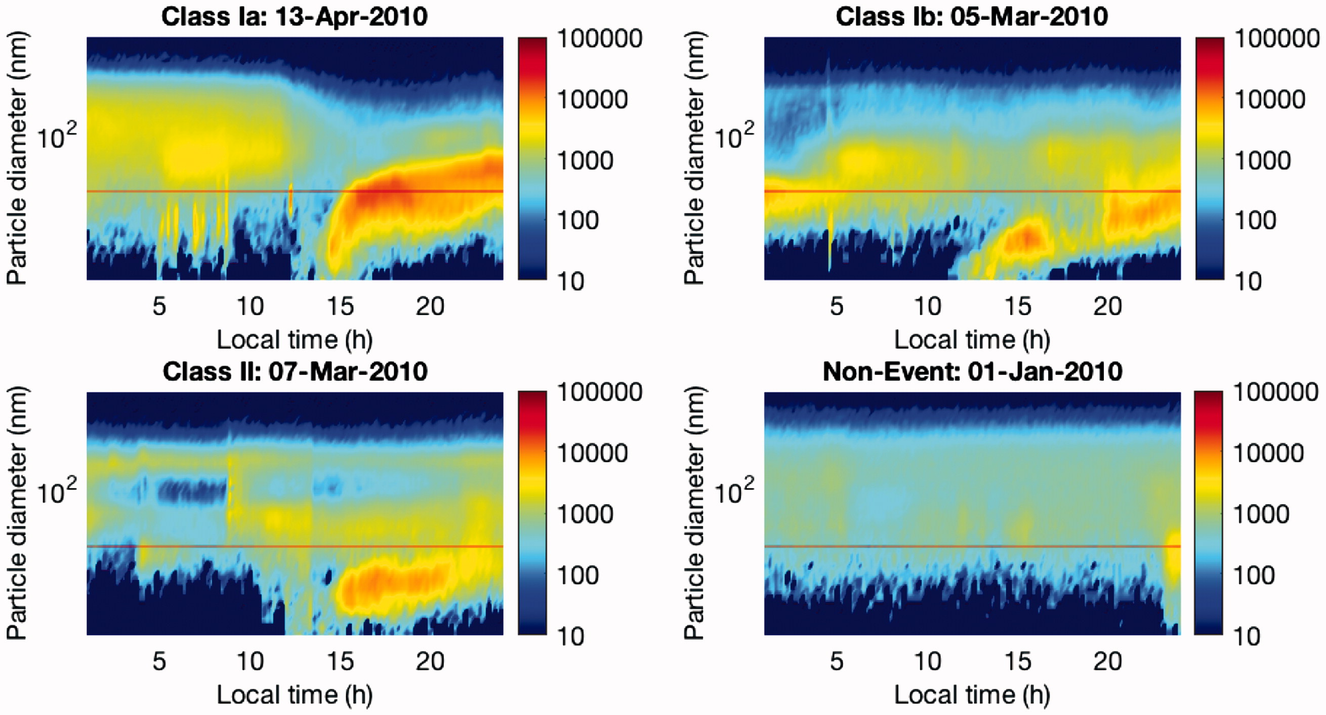
Fig. 2.
Four different types of NPF days, classified based on the method proposed by Dal Maso et al. (2005). The x-axis shows the 24-h time period, whereas y-axis represents the range of particle diameters (from 3 to 1000 nm). The color indicates the particle concentration (cm-3).
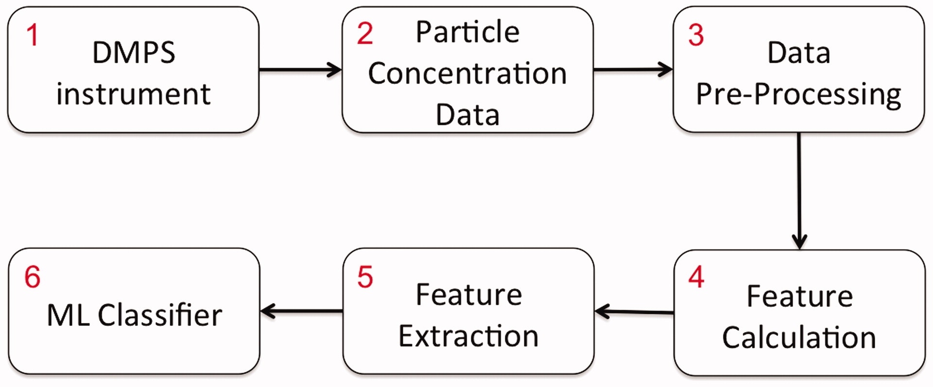
Fig. 3.
Schematic diagram of the ML methodology for classifying aerosol particle formation days.
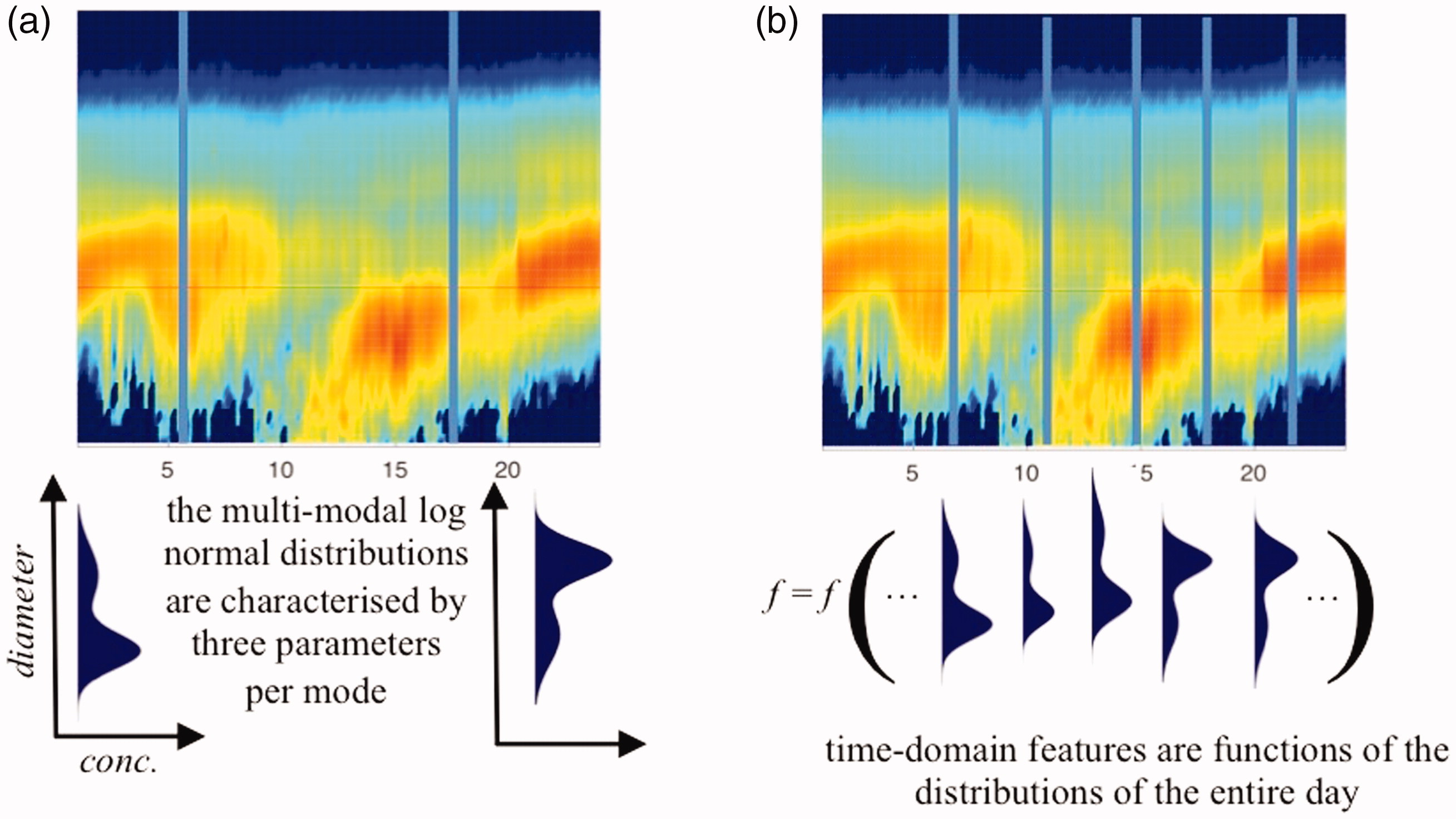
Fig. 4.
From the concentration data, two types of features are calculated to be used in the learning and validating of the neural network. At each instance of time, the ambient aerosol particle distribution can be presented as a multi-modal log normal distribution, characterized by three parameters per mode (see panel (a)). The set of these fitted parameters are used as the first type of features given to the neural network. The ambient particle distribution evolves throughout the day and this change is manifested in the parameters of the log normal distributions. A set of time-domain quantities calculated over the entire measurement day (excluding nighttime) are given to the neural network as second type of features (see panel (b) and Table 1).
Table 1.
Time-domain feature representations used in this study. The notation of x(i) and N denote the signal x(i) at time i and the number of data points, respectively. In this case, the signal is equivalent with the concentration level of every particle size distribution.
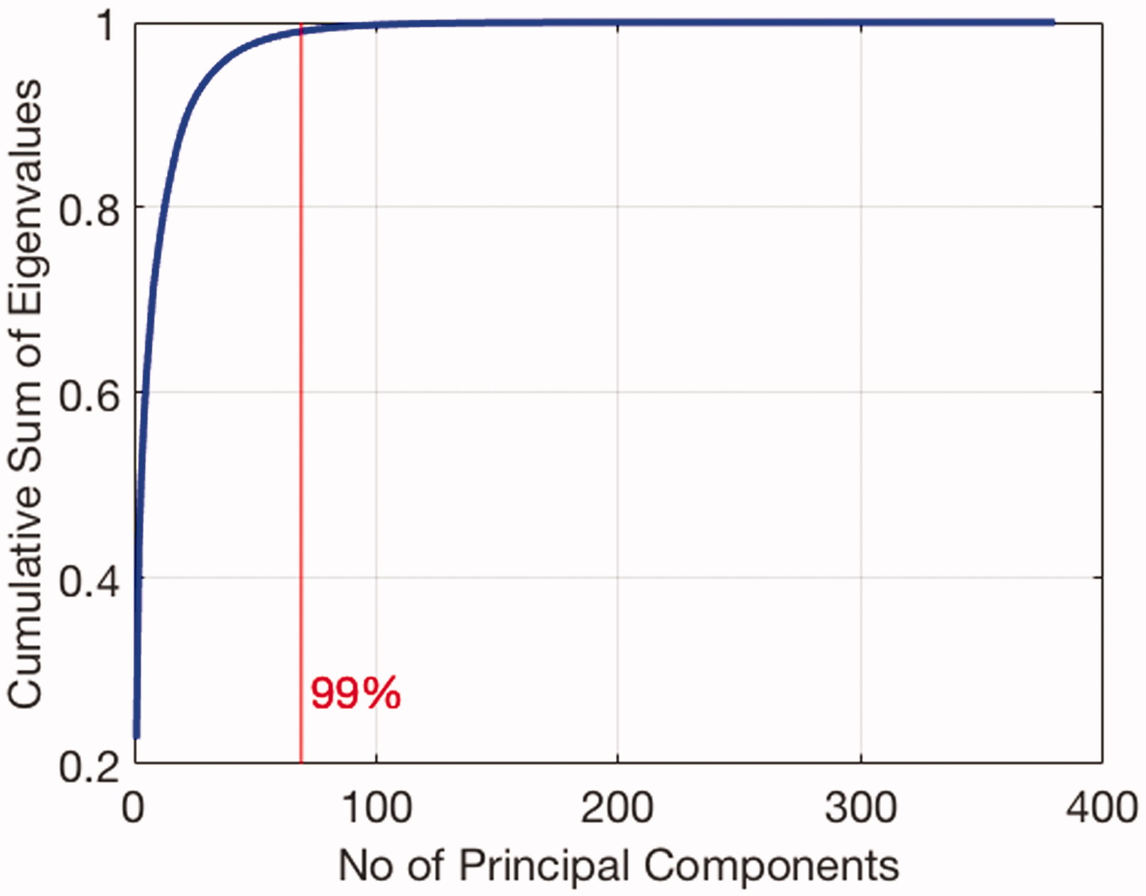
Fig. 5.
The cumulative sum of eigenvalues of the data in Principal Component (PC) space. In order to retain 99 per cent of original data information, we need to select only the first 69 PCs from almost 400 calculated features.
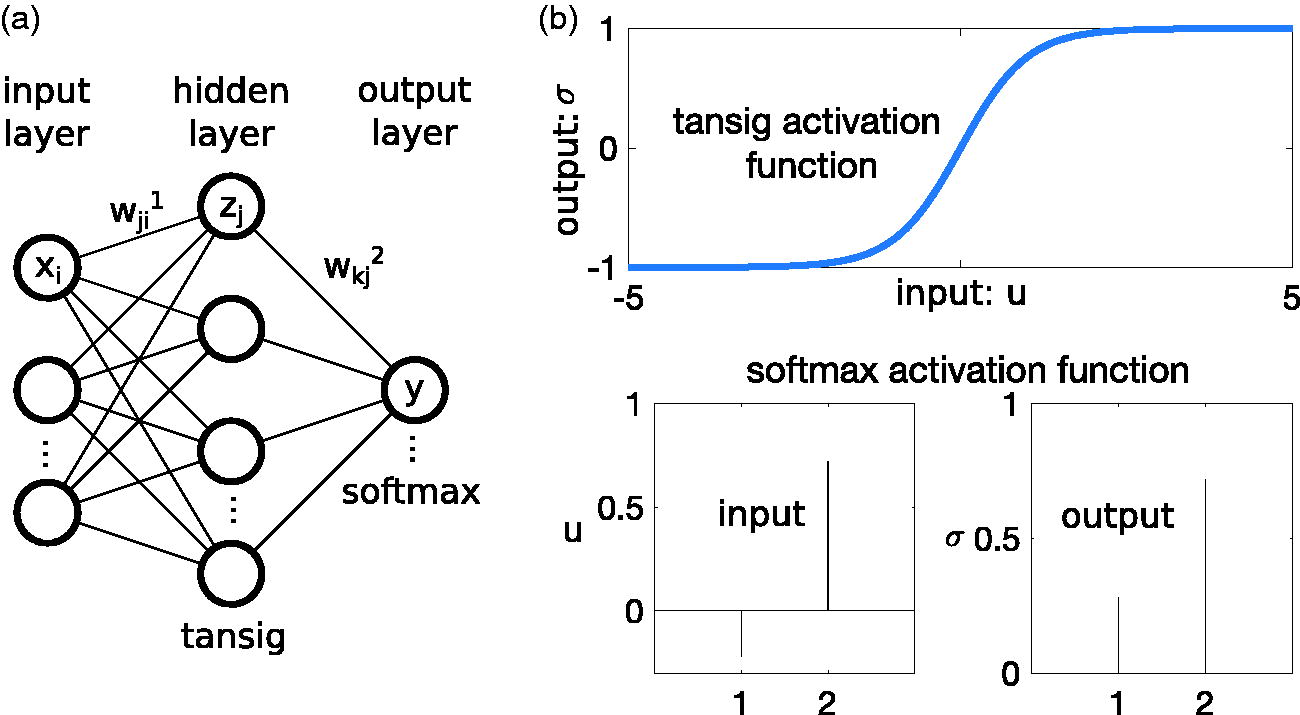
Fig. 6.
Schematic representation of a BNN with one hidden layer (a) and the used activation functions (b).
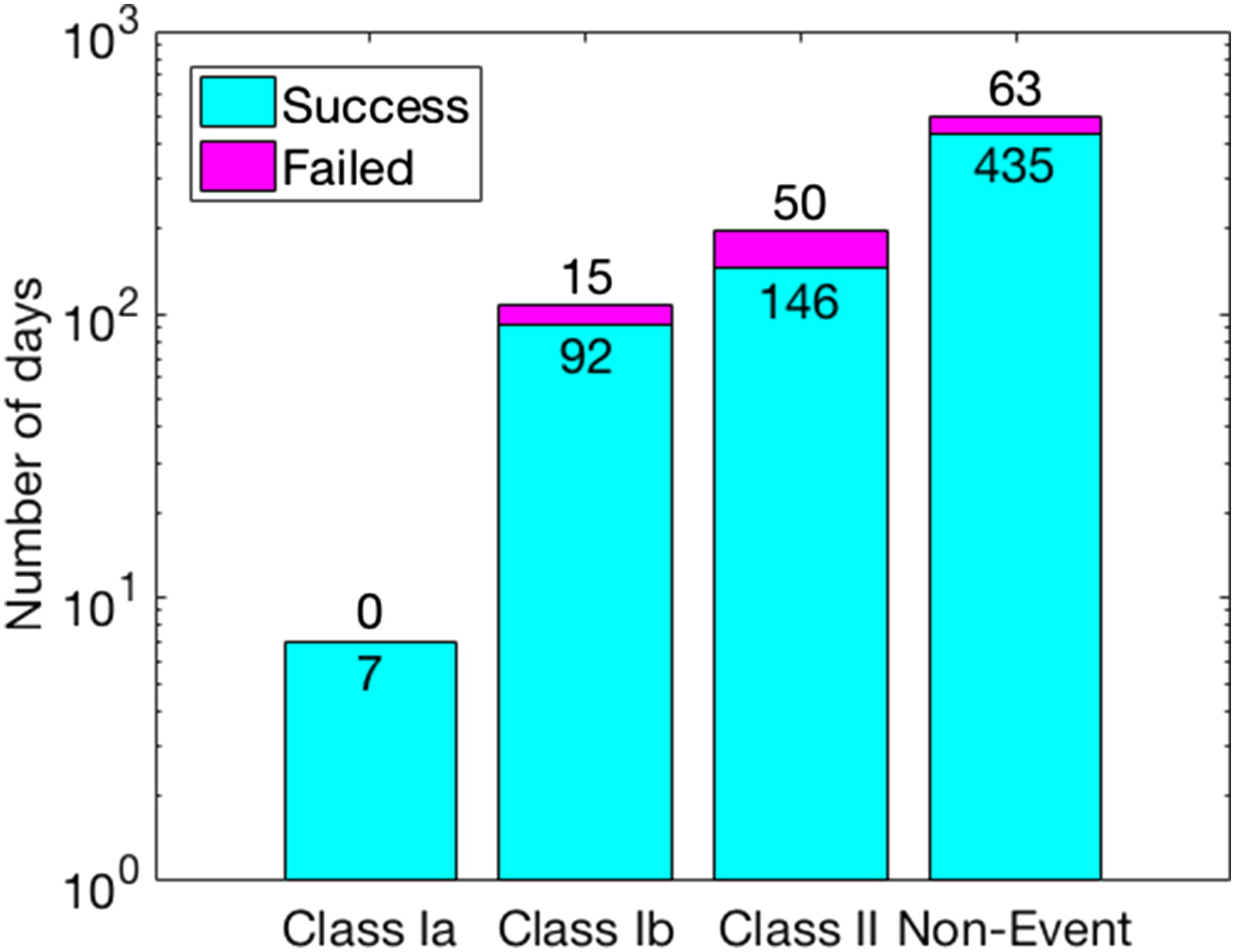
Fig. 7.
The bar chart of the successful and unsuccessful number of predicted days.