

Fig. 1.
Box-model simulations along a trajectory passing through the location of an ozone sonde observation of 14 ppb on 74 hPa (391 K potential temperature) at South Pole on 24 September 2003 (Grooß et al., 2011; Müller et al., 2018). The different panels show a time series of the most important parameters: (a) temperature of the air parcel, (b) PSCs: surface area density of ice (magenta, scaled by 0.1), NAT (green, scaled by 5) and liquid aerosol particles (blue), (c) ClOx (blue), and HCl (red), (d) ClONO2, and (e) ozone (note the logarithmic y-axis). Ozone and ClOx mixing ratios are shown as 24 hour averages.

Fig. 2.
Sensitivity simulations on the impact of the gas-phase reaction CH3O2 + ClO (R6) and the heterogeneous reaction HOCl + HCl (R2) on ozone loss. Top panel shows the simulated surface areas of NAT and liquid particles (also shown in Fig. 1). The panels below show HCl (b), active chlorine (ClOx, c), and ozone (d). Red line is the standard run (case A), blue line a run neglecting R6 (case B), green line a run neglecting R2 (case C), and orange line a case neglecting both R2 and R6 (case D). Ozone and ClOx mixing ratios are shown as 24 hour averages.
Table 1.
Sensitivity simulations on the impact of the gas-phase reaction CH3O2 + ClO and the heterogeneous reaction HOCl + HCl on ozone loss.

Fig. 3.
The temporal development of CH2O (panel a), HO2 (panel b), and CH3O2 (panel c) for the standard run (case A, red lines) and for case B (blue lines) neglecting R6.
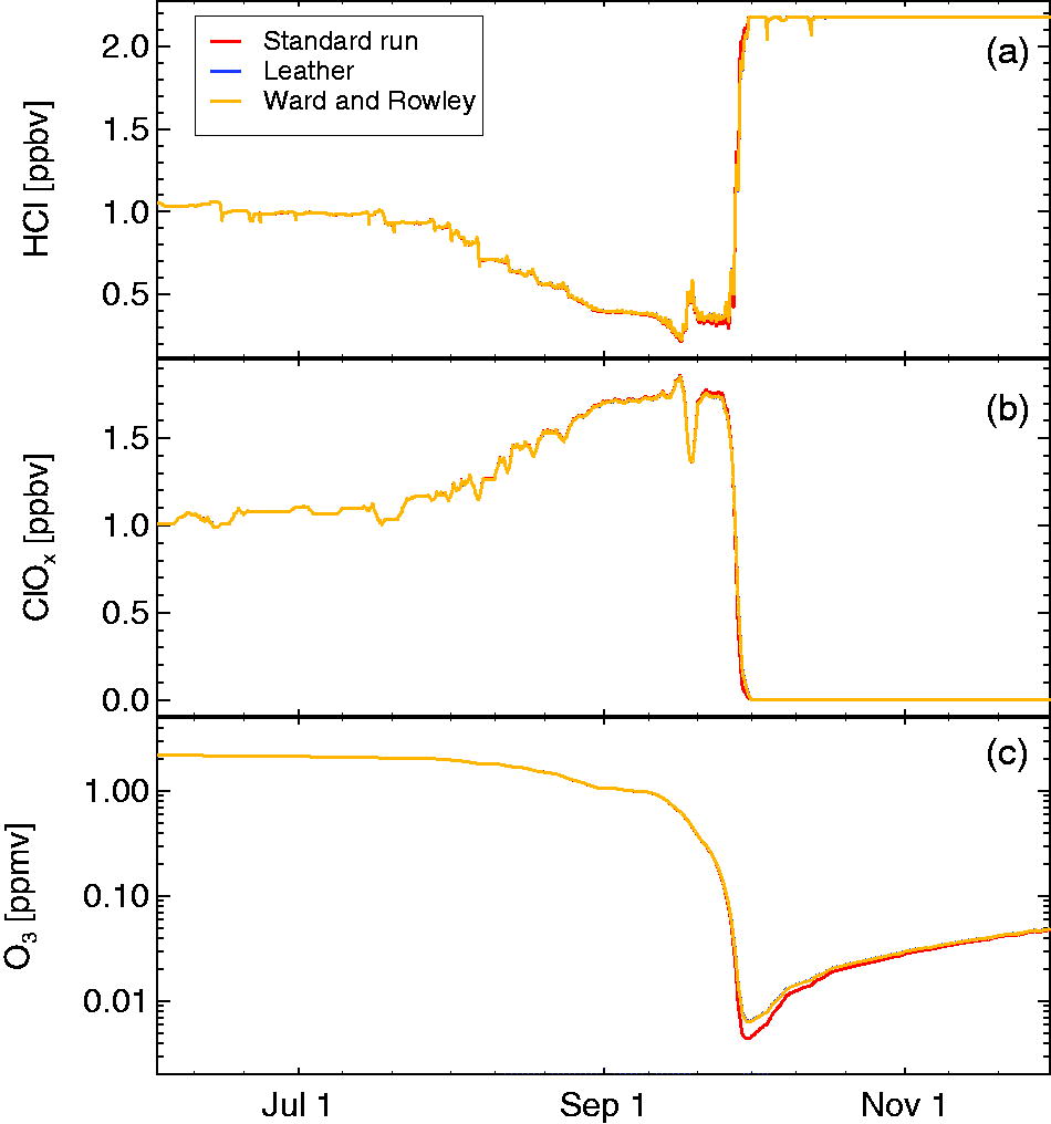
Fig. 4.
Sensitivity simulations on the rate constant of reaction R6 (CH3O2 + ClO). The panels show HCl (a), active chlorine (ClOx, b), and ozone (c). Red line shows the standard run using the recommended value (Sander et al., 2011) for R6, blue line shows a run assuming the overall rate constant for R6 reported by Leather et al. (2012) and the yellow line indicates the rate constant for R6 reported by Ward and Rowley (2016). (The blue and the yellow lines are almost identical.) Ozone and ClOx mixing ratios are shown as 24 hour averages.

Fig. 5.
Sensitivity simulations including CH3OCl chemistry. The panels show HCl (a), active chlorine (ClOx, b), and ozone (c). Red line shows the standard run. The blue, green, and orange lines show runs assuming 100% efficiency for the production of CH3OCl in the branching ratio of R6/R7. The blue line shows results from a run assuming loss of CH3OCl only through photolysis, the green line results assuming in addition loss through the reaction of with the products and the orange line assuming in addition loss through the reaction of , but with the products . Ozone and ClOx mixing ratios are shown as 24 hour averages.

Fig. 6.
Sensitivity simulations including CH3OCl chemistry. The panels show HCl (a), active chlorine (ClOx, b), and ozone (c). Red line shows results for the standard run. Blue line shows results for a run assuming realistic branching ratios for CH3OCl production in R7 and for HCl production in R18 (see text). Ozone and ClOx mixing ratios are shown as 24 hour averages.
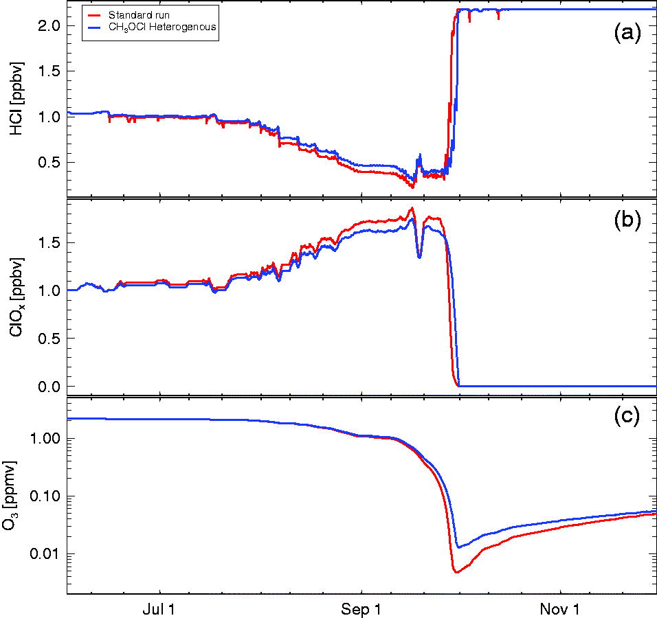
Fig. 7.
Simulations assuming the hypothetical heterogeneous reaction → (Kenner et al., 1993; Crowley et al., 1994); the sensitivity run assuming that this reaction occurs on ice, NAT and STS is shown in blue and the standard run is shown in red. The panels show HCl (a), active chlorine (ClOx, b), and ozone (c). Ozone and ClOx mixing ratios are shown as 24 hour averages.

Fig. 8.
Results of the temporal development of methylhypochlorite (CH3OCl, panel a) and methanol (, panel b). Shown are results for a case (blue line) with a realistic formation rate of CH3OCl in reaction R7 and a realistic branching ratio for the reaction (reactions R17 and R18). Also shown are results for a run with realistic assumptions for CH3OCl chemistry and, in addition, assuming that the hypothetical heterogeneous reaction R22 occurs in the polar stratosphere (black lines). The methanol mixing ratios for the standard run are shown as the red line in panel b.
Table 2.
The set of additional reactions taken into account to describe the chemistry of .
[i] Top part shows the reactions and the reported rate constants from the literature, bottom part shows the reactions and rate constants as implemented (both for the 50:50 and the 20:80 branching ratio of R25 and R26) in the chemistry scheme employed here (Maricq et al., 1994).
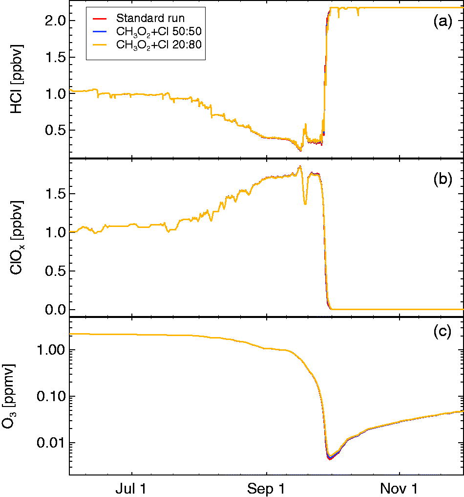
Fig. 9.
Simulations including the reaction products. The panels show HCl (a), active chlorine (ClOx, b), and ozone (c). The two branching ratios of this reaction and three decay channels for CH2O2 are taken into account (see Table 2 for the details of the reactions implemented in the chemistry scheme). Ozone and ClOx mixing ratios are shown as 24 hour averages.