
Table 1.
An overview of the model and observation based CO2 component estimates. All observation-based estimates (obs*) calculate the CO2 background with a 45-day REBS, and translate CO above a similar CO background estimate with the designated . All modeled estimates were calculated with FLEXPART-COSMO and the data product listed.
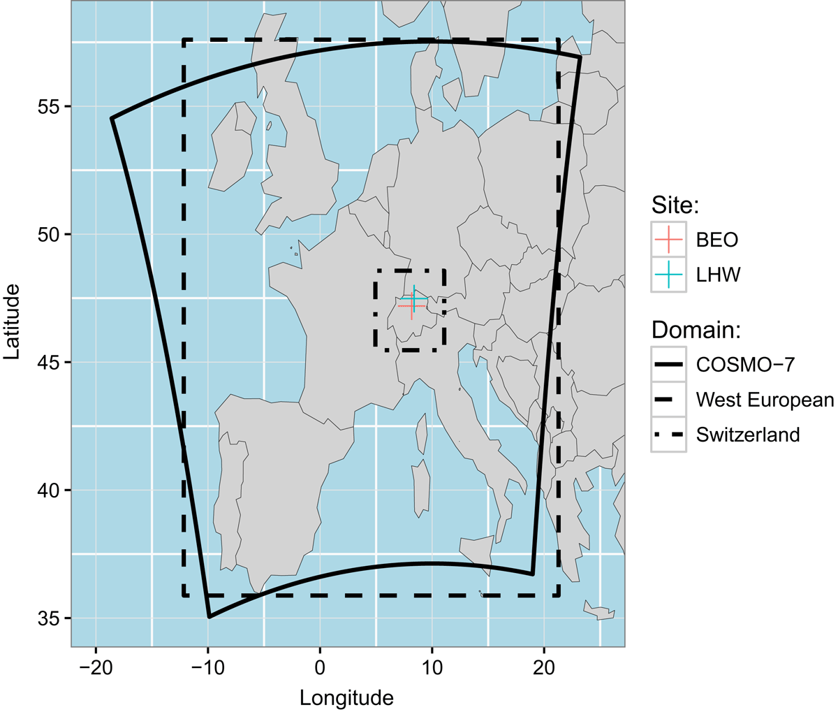
Figure 1.
Simulation domains of this study. The COSMO-7 represents the driving meteorology. The west European and Switzerland domains comprise the areas where surface sensitivity and flux influence is calculated for the past 4 days to simulate regional signals. Outside these temporal and spatial domains the initial mole fraction is taken as the background signal.
Table 2.
Simulation characteristics for two observation sites of the CarboCount CH network. Listed from left to right are observation heights (m above ground level), FLEXPART-COSMO particle release heights (m above model ground level), the ‘true’ site altitudes (m above sea level), smoothed COSMO numerical weather prediction model’s (4 km) site altitude, and the geographic site locations.
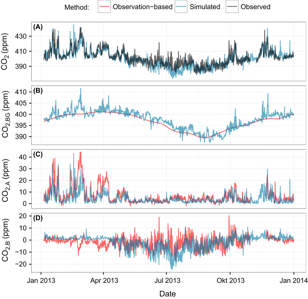
Figure 2.
Observed CO2 mole fractions (A), observation-based (obs1) and FLEXPART-COSMO-modeled (mod1) CO2 background (B), anthropogenic (C) and biospheric (D) components at Beromünster during 2013. Also shown in (A) is the sum of all simulated components. For an overview of the settings for obs1 and mod1 see Table 1.
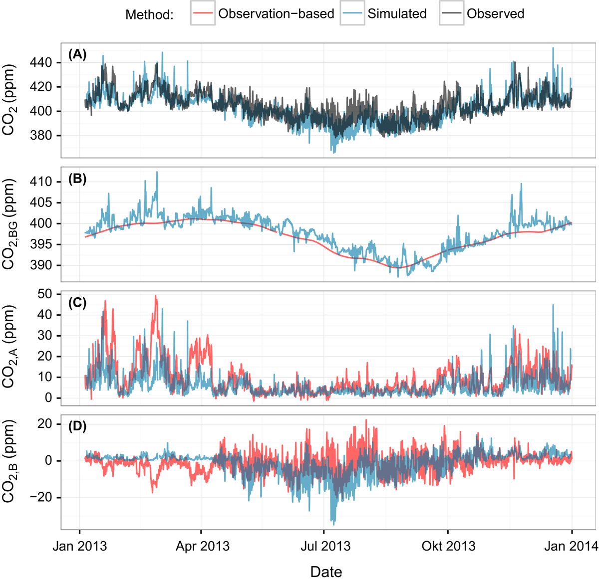
Figure 3.
Same as Fig. 2 but at the Lägern-Hochwacht site.
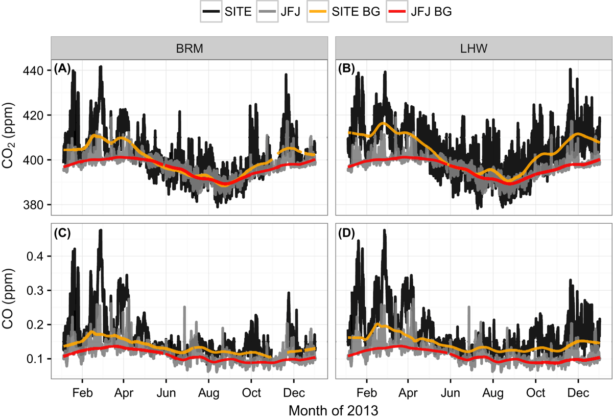
Figure 4.
CO2 (panels A–B) & CO (panels C–D) measured mole fractions (black and gray) and ‘robust estimate of baseline signal’ (REBS) estimates (red and orange) at Beromünster, Lägern-Hochwacht, and Jungfraujoch (JFJ) during 2013. The REBS background estimates are calculated with a 45-day local regression window.
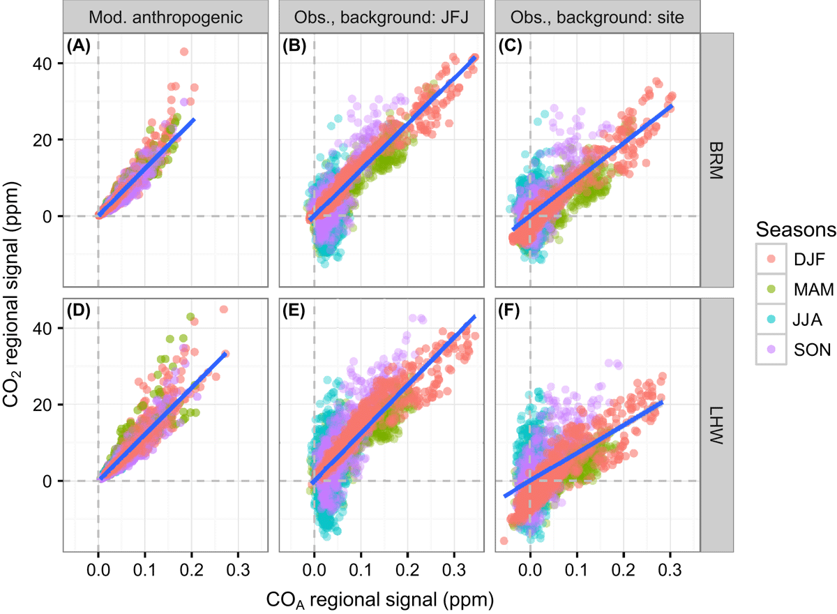
Figure 5.
Modeled and measured CO2 and CO regional signals at Beromünster and Lägern-Hochwacht, colored according to season. Panel A: modeled CO2,A and COA at Beromünster. The slope of the regression line corresponds to of method mod1. Panel B: CO2, R and COA regional signals above a background signal from Jungfraujoch. The slope of the regression line is calculated using only wintertime regional signals and corresponds to of method obs1. Panel C: the same is shown as in panel B except using background estimates from the target site Beromünster (method obs5). Panels D-F: the same as panels A–C shown with regional signals from Lägern-Hochwacht.
Table 3.
Sensitivity of the inverse ratios ( ppb CO/ppm CO2) to the choice of background signal, and to the choice of local regression window width. The uncertainty of is reported as the confidence interval of the slope from the total weighted least squares regression, forced through the origin. is the coefficient of determination estimated by Pearson’s correlation. The obsN cases included observations from the large-scale pollution event at the end of February, whereas the obsN cases used only the observations during this and a similar event in March/April (see Fig. 6 and Section 4.3).
Table 4.
Summary of observed ’s found in previous studies. The upper portion of the table displays long-term observation results, and the lower half of the table displays observation campaign results. COA/CO2,R refers to ratios calculated from continuous CO2 and CO observations above background, analogous to this study. COA/CO2, FF indicates fossil fuel CO2 (CO2, FF) calculated from (see Levin et al. 2003). The information used for the method is presented as the apparent ratio calculation, background, and the metric shown. The units of are ppb CO/ppm CO2.
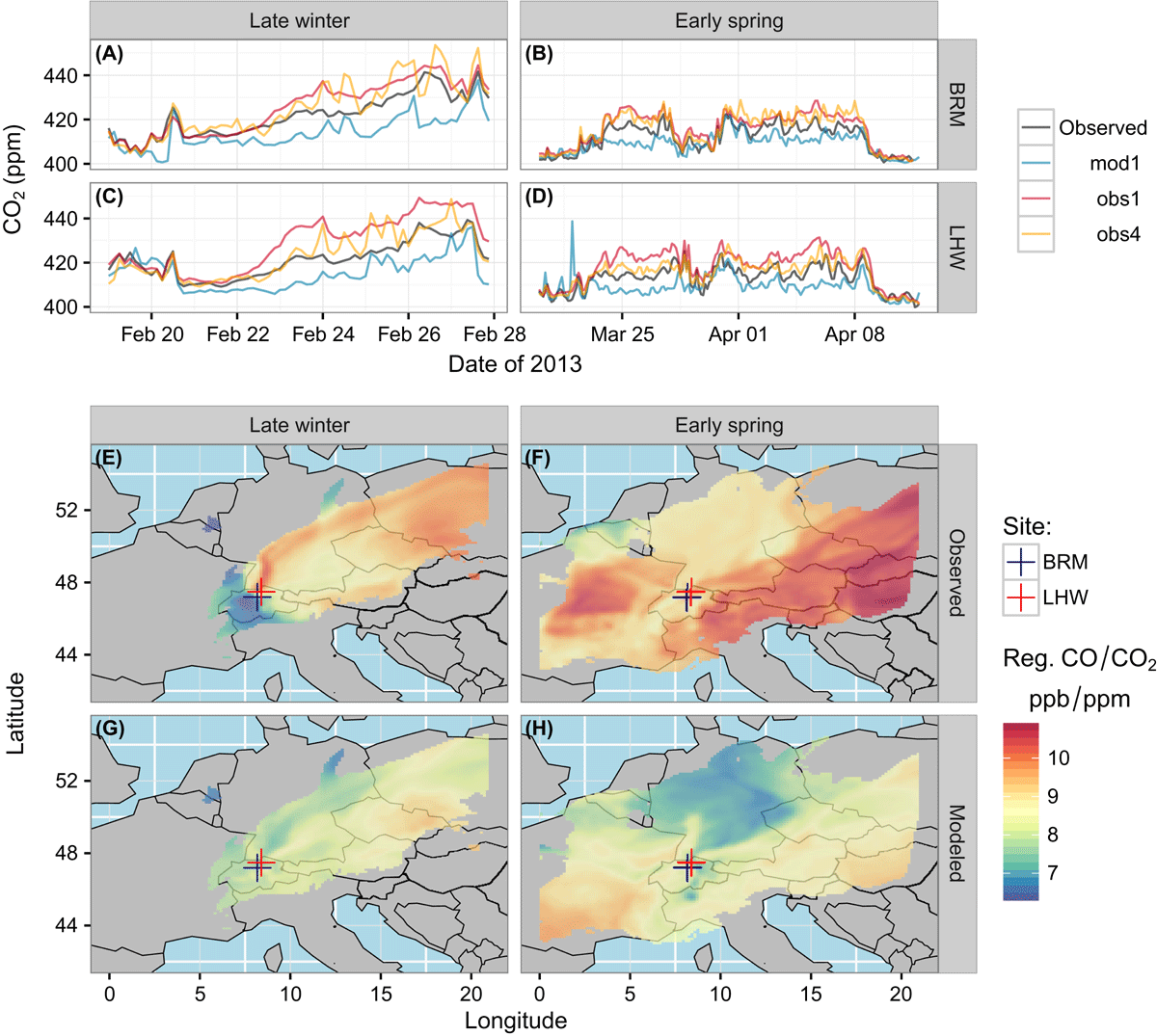
Figure 6.
Spatially disaggregated modeled and observed regional CO : CO2 ratios for late winter- and springtime pollution events during which neither observation-based nor modeled estimates explain the observed CO2 at Beromünster and Lägern-Hochwacht. The disaggregation followed the method by Stohl (1996) (see Section 4.3). It was only applied to surface sensitivities above a threshold which denotes an isoline enclosing 90 % of the cumulative sum of surface sensitivities (see Oney et al. 2015) from the respective time periods.
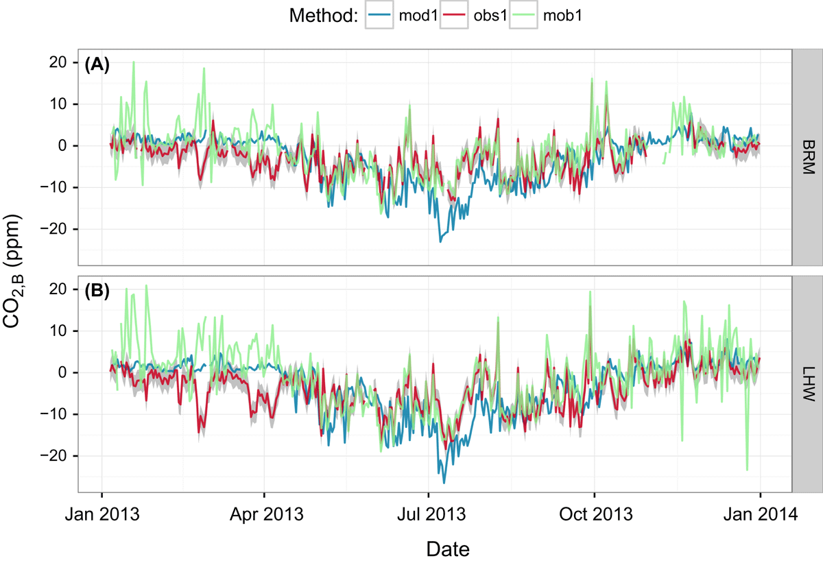
Figure 7.
Afternoon (1200–1500 UTC) biospheric CO2 signals at Beromünster and Lägern-Hochwacht during 2013. The modeled (mod1) and observation-based (obs1) biospheric signals (CO2,B) are also shown in panel D of Figs. 2 & 3. The model-based residual biospheric signal (mob1) is the residual of measured CO2 after subtracting the modeled background and anthropogenic signals. The uncertainty (gray) enveloping the residual biospheric signal (obs1) accounts for the uncertainty introduced by the observation based background and anthropogenic CO2 signals.
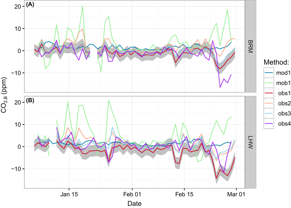
Figure 8.
Comparison of biospheric CO2 signals (CO2,B) at Beromünster (panel A) and Lägern-Hochwacht (panel B) during the period of 2013-01 – 2013-03.
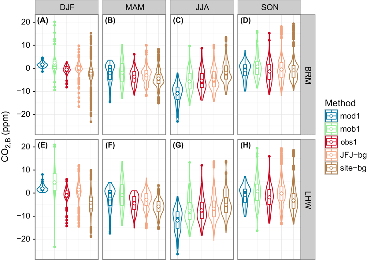
Figure 9.
Comparison of the statistical distributions (box and violin [kernel density] plots) of afternoon (1200–1500 UTC) CO2 biospheric signals at Beromünster (panels A–D) and Lägern-Hochwacht (panels E–H) during 2013, summarized by season for each method (Table 1). JFJ-bg and site-bg denote the distributions of all biospheric signals resulting from the site’s or Jungfraujoch REBS (JFJ-bg includes obs1), respectively. The mean of each distribution is marked by a diamond. The model-based residual biospheric signal (mob1) is the residual of measured CO2 after subtracting the modeled background and anthropogenic signals.
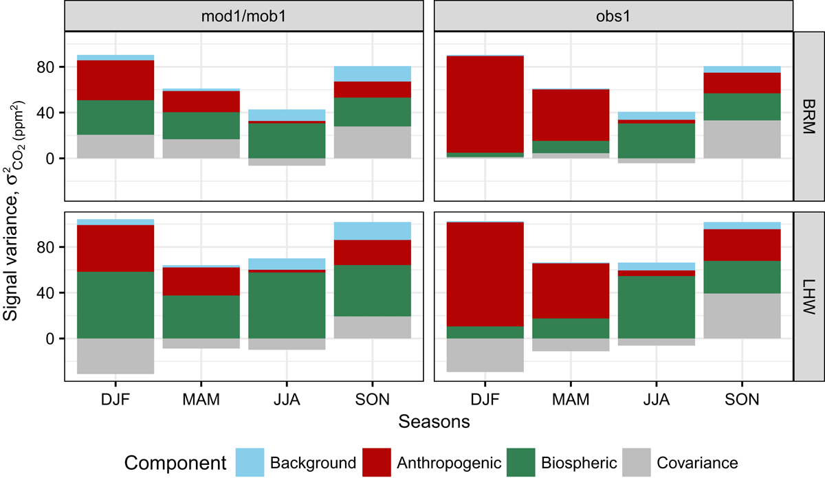
Figure 10.
Afternoon (1200–1500 UTC) CO2 signal variances at Beromünster and Lägern-Hochwacht during 2013. The model-based CO2 signal variances (mod1/mob1) are calculated from the respective anthropogenic, biospheric, and background components. The covariance contribution included in the figure gives the sum of the three covariances between the three components. The model-based residual biospheric signal (mob1) is used instead of the modeled biospheric signal (mod1) to be comparable with the observation-based residual biospheric signal (obs1).
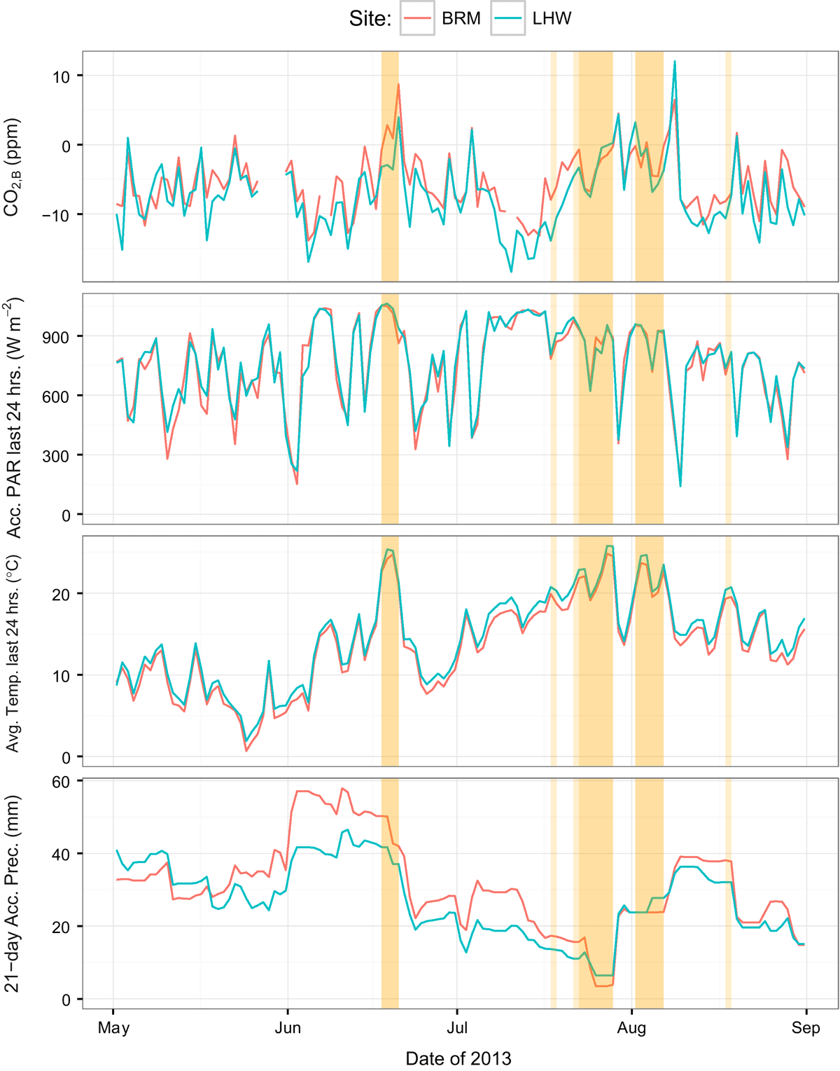
Figure 11.
Observed afternoon (1200–1500 UTC) biospheric CO2 signals (obs1) along with temperature (average of past 24 hours), photosynthetically active radiation (PAR) accumulated over the past 24 hours, as well as precipitation accumulated over the previous 21 days (as a proxy of soil moisture), during the main growing season (01 May–01 September) of 2013 interpolated from COSMO-2 analysis fields to the observation site positions, Beromünster and Lägern-Hochwacht at 250 m above model ground level. Shaded areas demarcate periods during which the average temperature of the preceding 24 hours was C.
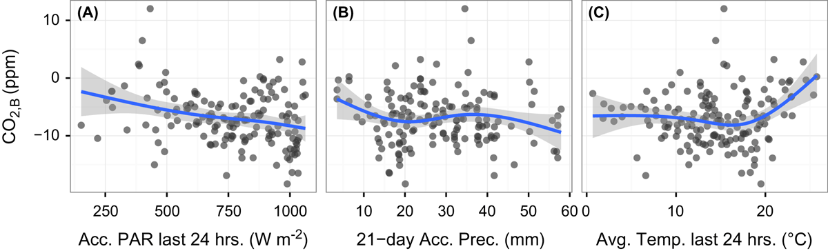
Figure 12.
Response of observed afternoon (1200–1500 UTC) biospheric CO2 signals (obs1) to modeled (described in Fig. 11) PAR, accumulated precipitation, and average temperature at both Beromünster and Lägern-Hochwacht during the growing season (01 May–01 September) of 2013. We narrowed our investigation to convective meteorological situations according to the categorization by Weusthoff (2011). The blue line corresponds to a generalized additive model binned by the 95 % confidence interval.