
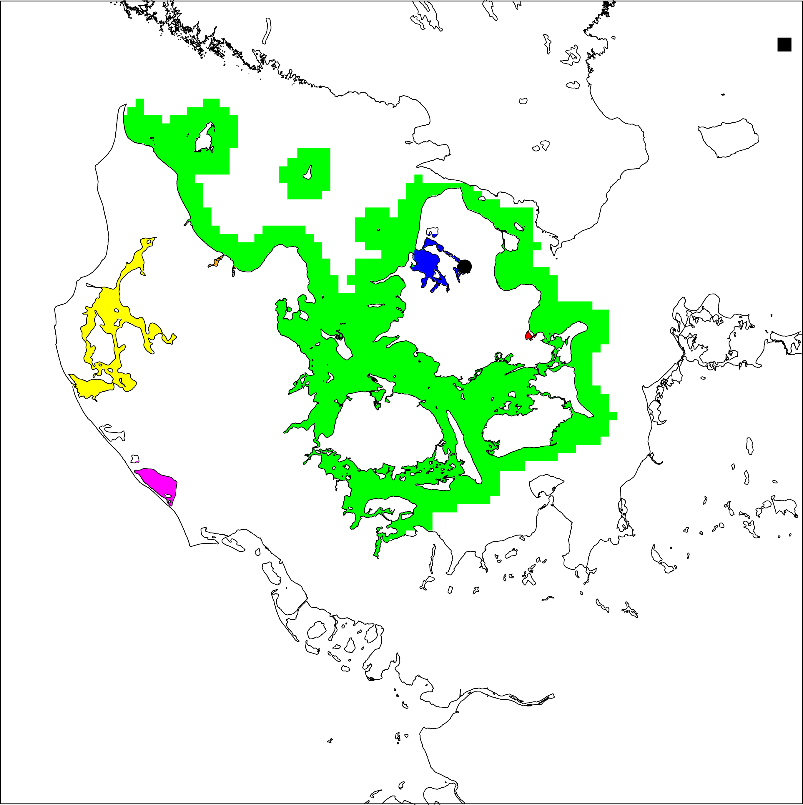
Figure 1.
Subdivision for the Danish inner waters and coastal areas. Blue: Roskilde Fjord, 430 km. Green: Danish inner coast, 23,421 km. Yellow: Limfjorden, 1538 km. Orange: Mariager Fjord, 59 km. Red: Præstø Fjord, 15 km. Magenta: Rinkøbing Fjord, 206 km. The Risø site is marked with , while the BY5 site is denoted by .
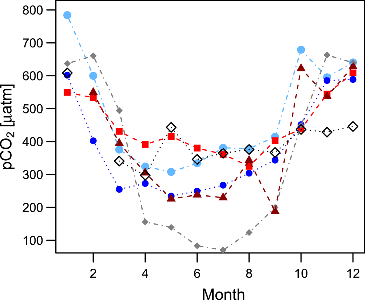
Figure 2.
Coastal Danish inner waters monthly p climatologies for the six subdivisions:  Roskilde Fjord,
  Danish inner Coast,
  Limfjorden,
  Mariager Fjord,
  Præstø Fjord,
  Ringkøbing Fjord .
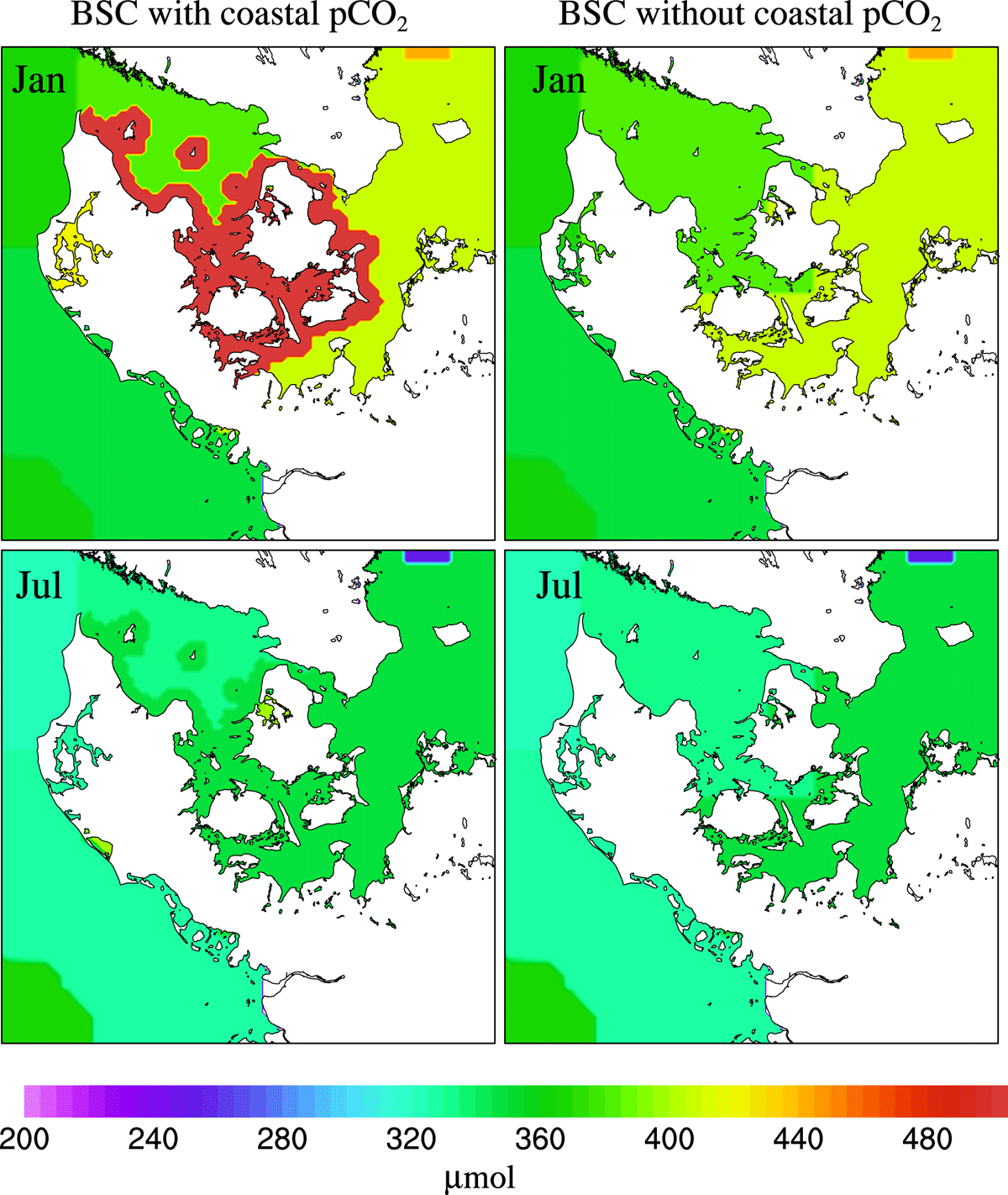
Figure 3.
January and July examples of the p maps used for the Danish coastal area. Both are based on the BSC climatology. The left panels also include the improved coastal p for the Danish inner waters.
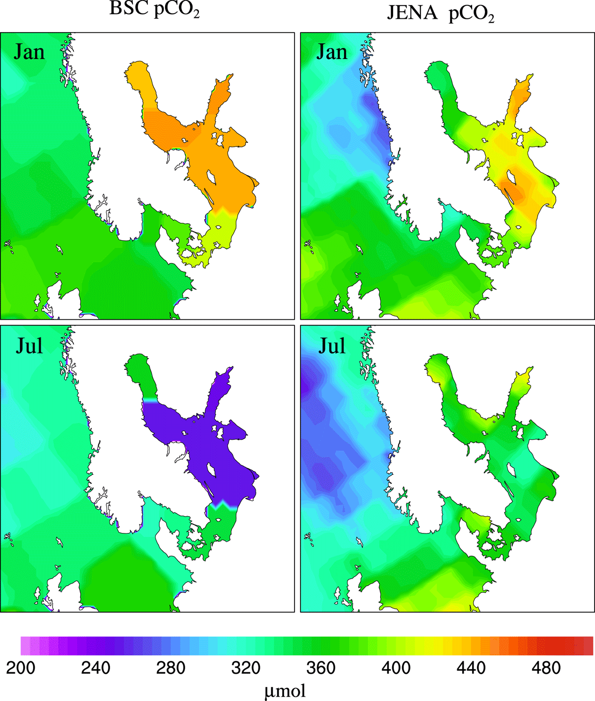
Figure 4.
January and July examples of the different p maps used for the Baltic Sea. Left panel contains the BSC, while right panel contains monthly means from the JENA p surface product.
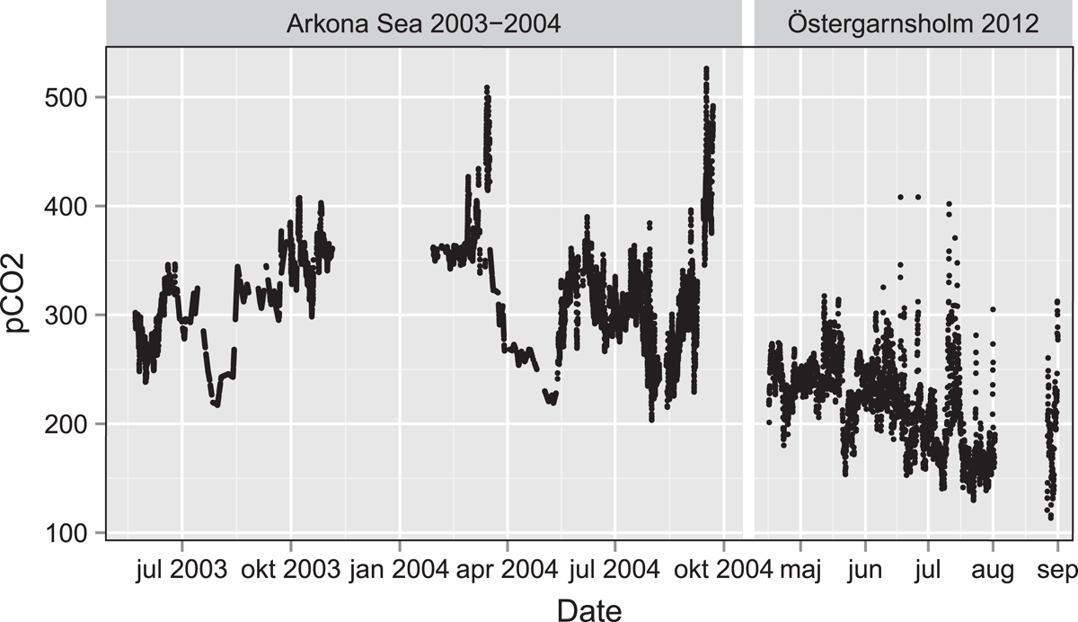
Figure 5.
Continuous measurements of surface water p from the Arkona Sea platform and the Östergarnsholm site.
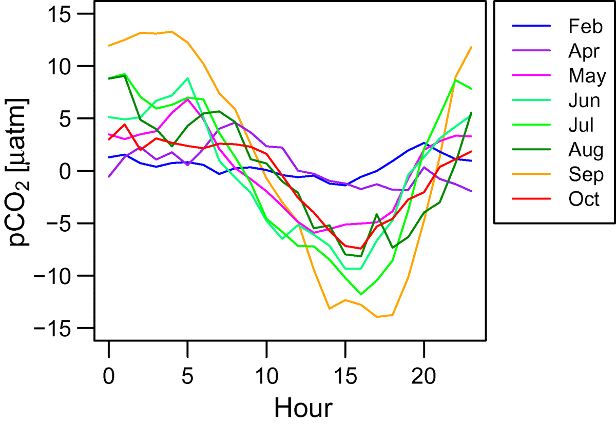
Figure 6.
Calculated averaged monthly diurnal cycles of surface water p.
Table 1.
List of simulations. Abbreviations are used for the simulation names and refer to the temporal resolution of p: v:variable, c:constant monthly, a:atmosphere, m:marine. BSC is an abbreviation of the Baltic Sea Climatology, while JENA corresponds to the surface p product developed by Rödenbeck et al. (2013) and Rödenbeck et al. (2014).
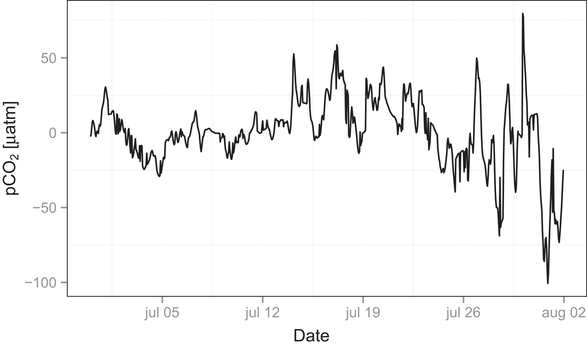
Figure 7.
Actual variability of surface water p measured at the Arkona Sea platform during July 2004.
Table 2.
Monthly means of the air–sea flux for the Baltic Sea and the Danish inner waters (GgC month). The last column shows the net annual flux (GgC yr). A positive sign indicates the release of from the ocean to the atmosphere, while a negative sign indicates the uptake of atmospheric by the ocean.
Table 3.
Annual means, differences and percentage change for the Baltic Sea and Danish Inner waters. Annual means and differences are in GgC yr. Differences and percentage changes are calculated with vacm as the reference.
Table 4.
July monthly means, differences and percentage change for the simulations RV_vavm, vacm and vavm for the six sub-basins within the Baltic Sea and Danish inner waters. Monthly means and differences are in GgC month. The notation of difference and percentage changes are given as vacm, and vavm when indicating the difference and percentage change with respect to RV_vavm, while vacm_vavm is between these two simulations.
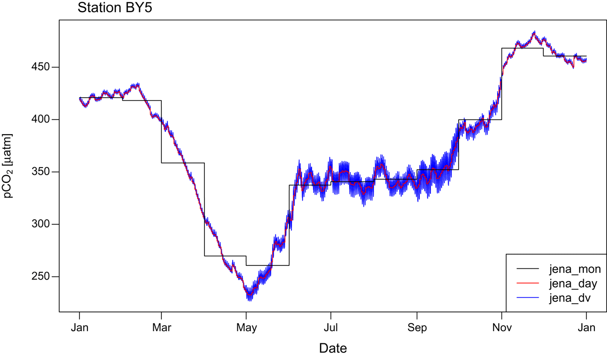
Figure 8.
The progression of surface water p during 2011 at the BY5 site for the simulations based on the JENA p product.
Table 5.
Seasonal uptake and release, annual means, differences and percentage change in the Baltic Sea and Danish inner waters for the JENA simulations. Differences and percentage changes are calculated with jena_mon as the reference. The units are in GgC yr.
Table 6.
Annual means, differences and percentage change for the Danish coastal areas using results from nest 4 of the DEHM. Annual means and differences are in GgC yr. Differences and percentage changes are calculated with vacm as the reference.
Table 7.
Monthly mean air–sea fluxes for the Danish coastal areas for the simulation vavm, including the improved coastal p (GgC month). The last column is the annual total flux(GgC yr).
Table 8.
Monthly mean air–sea fluxes for the Danish coastal areas for the simulation vavm, without improved coastal p (GgC month). The last column is the annual total flux(GgC yr).
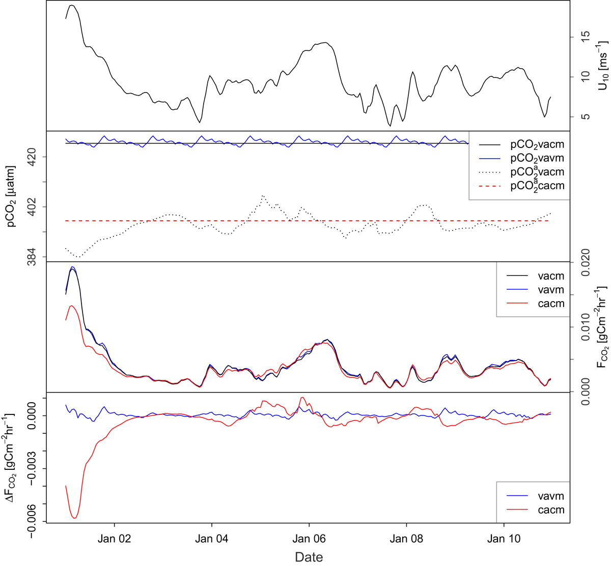
Figure A1.
January 2011 time series at the BY5 site for the simulations using the BSC. Top panel: wind speed,u applied in all the simulations. Upper middle panel: Marine p and atmospheric p, denoted pCO. Lower middle panel: air–sea exchange, . Bottom panel: Difference in air–sea exchange between the simulations, , calculated with vacm as the reference.
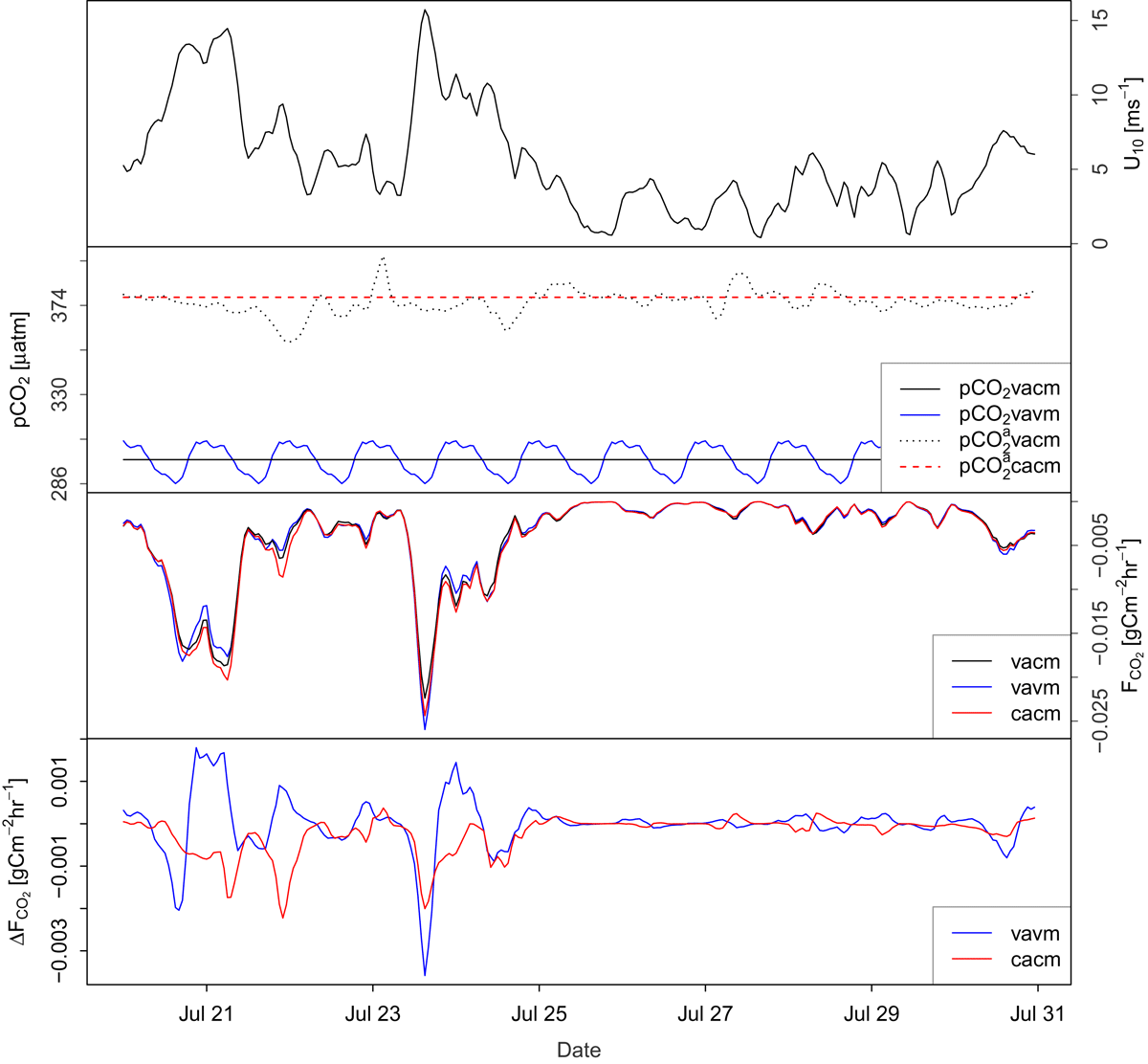
Figure A2.
July 2011 time series at the BY5 site for the simulations using the BSC. Top panel: wind speed,u applied in all the simulations. Upper middle panel: Marine p and atmospheric p, denoted pCO. Lower middle panel: air–sea exchange, . Bottom panel: Difference is air–sea exchange between the simulations, , calculated with vacm as the reference.
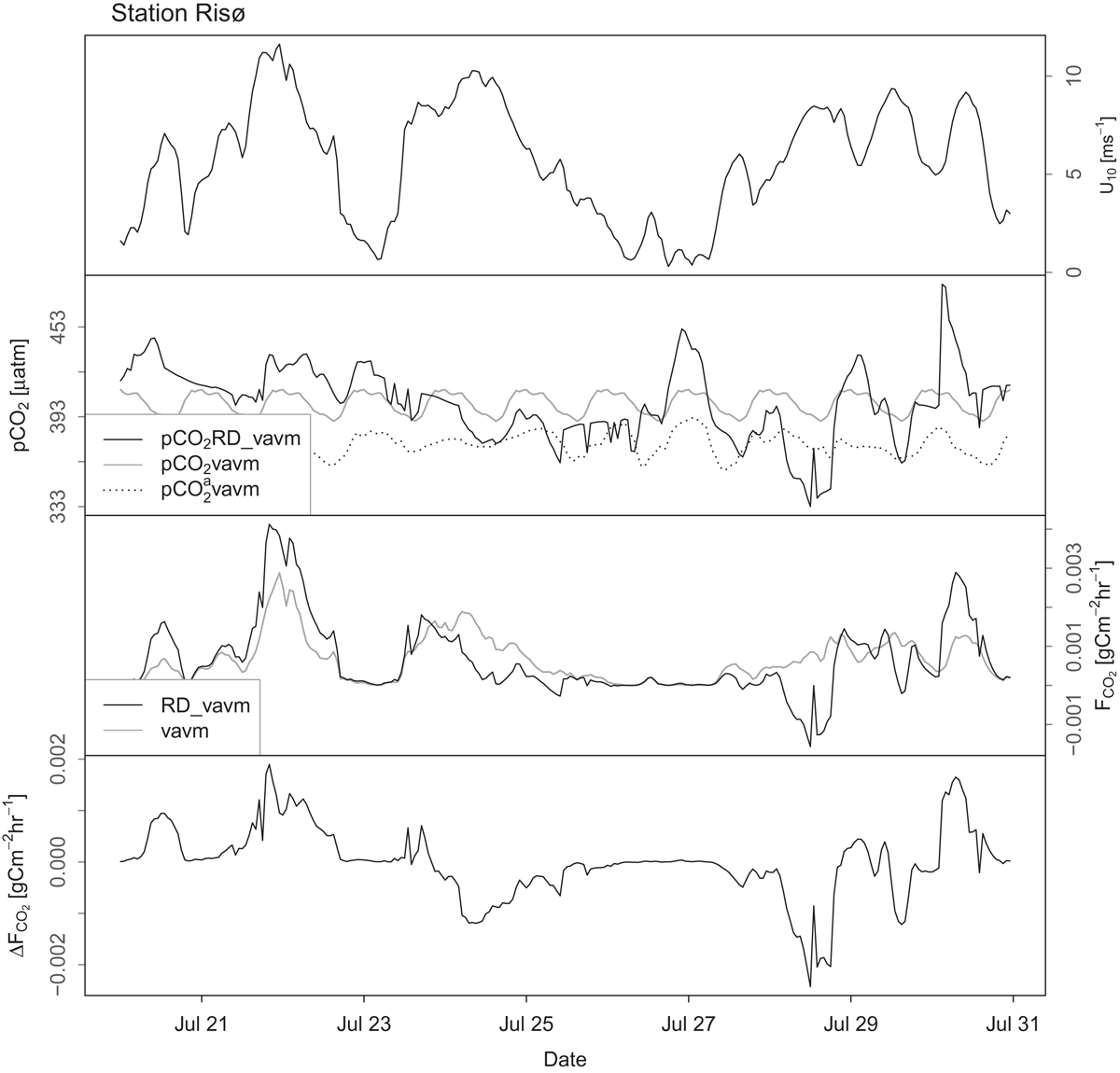
Figure A3.
July time series at the Risø site for RD_vavm and vavm. Top panel: wind speed, u applied in all the simulations. Upper middle panel: Marine p and atmospheric p, denoted pCO. Lower middle panel: air–sea exchange, . Bottom panel: Difference in air–sea exchange between the simulations, , calculated as RD_vavm - vavm.
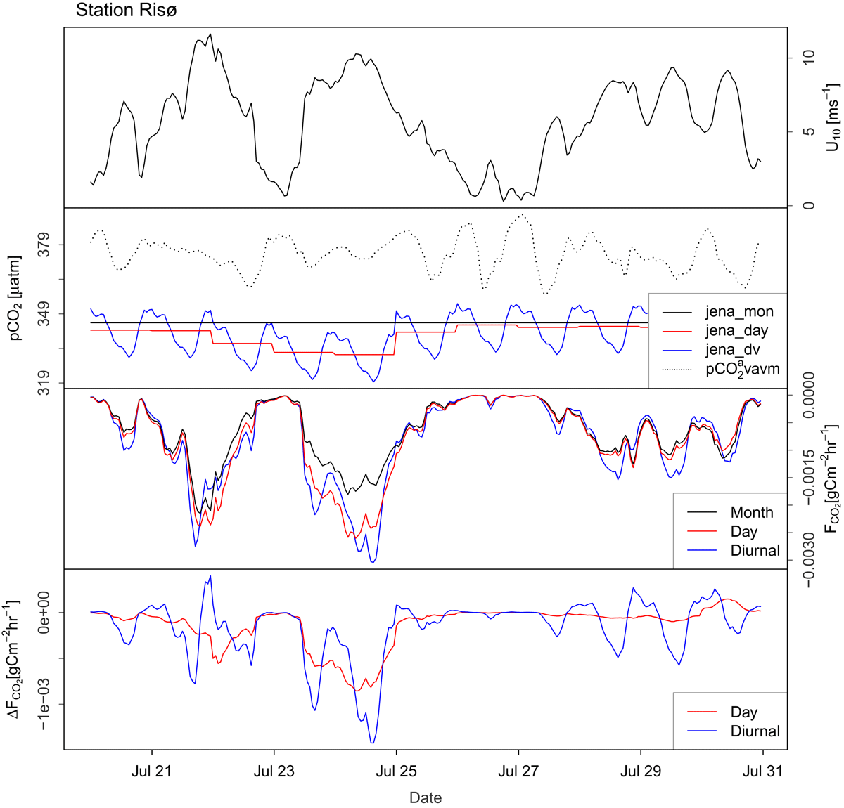
Figure A4.
July time series at the Risø site for the JENA simulations. Top panel: wind speed, u applied in all the simulations. Upper middle panel: Marine p and atmospheric p, denoted pCO. Lower middle panel: air–sea exchange, . Bottom panel: Difference in air–sea exchange between the simulations, , calculated with jean_mon as the reference.