
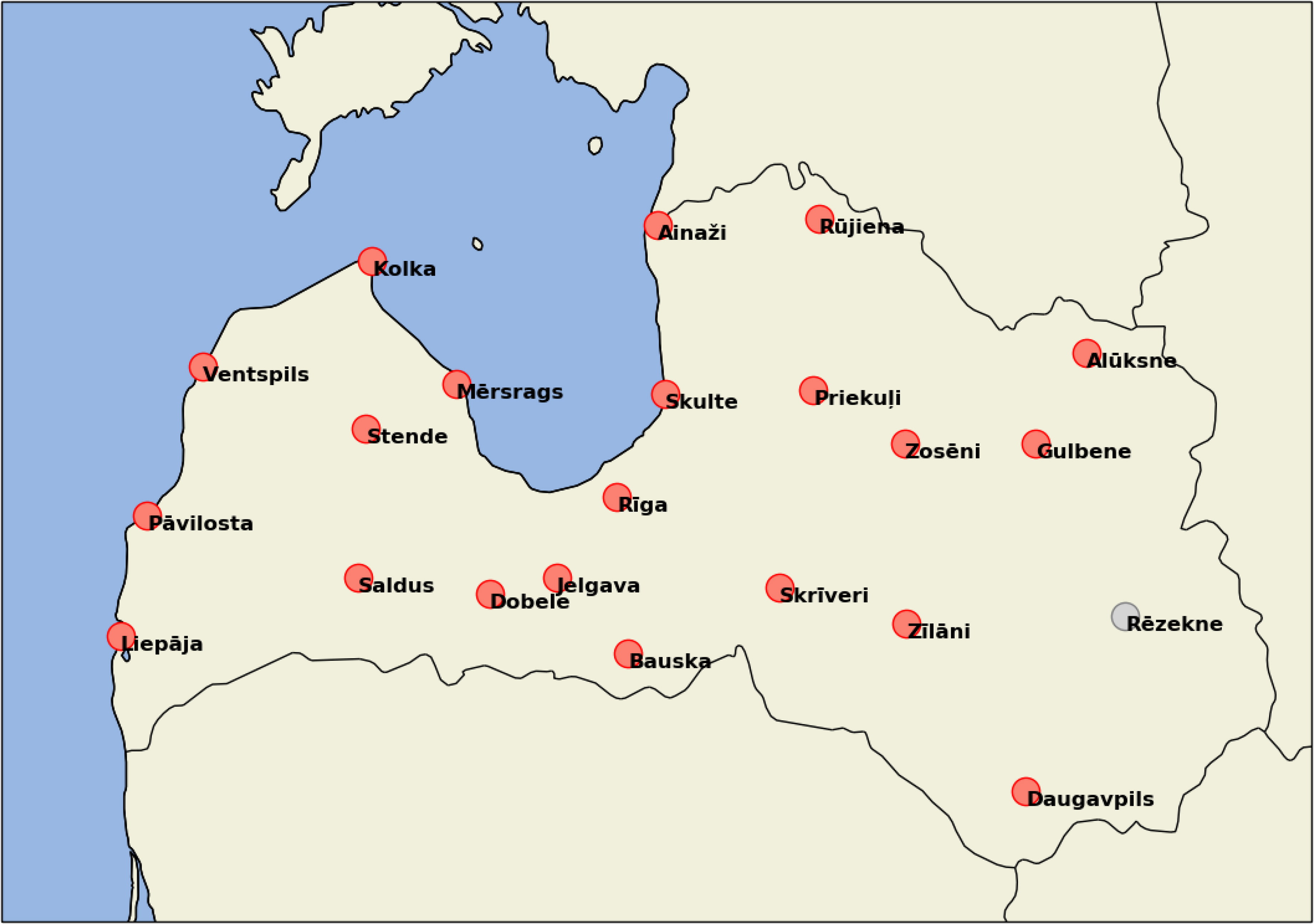
Fig. 1.
Locations of 22 observation stations in Latvia that record wind direction. Observation station Rēzekne (grey marker) was not used in further analysis, since it did not meet the data completeness criteria for the period of study (see text).
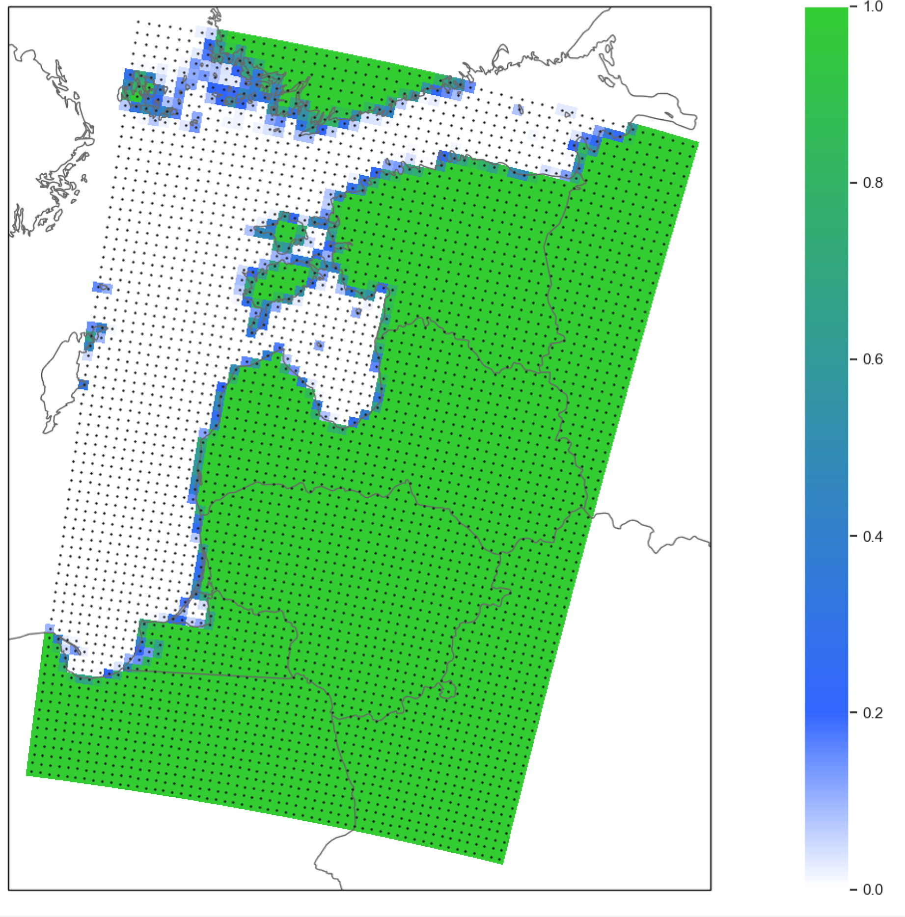
Fig. 2.
UERRA reanalysis data used in this study (56 × 80 gridpoints). Black dots indicate centres of gridpoints. Colours show model data for land/sea coverage of grid cells, 1 – land, 0 – sea.
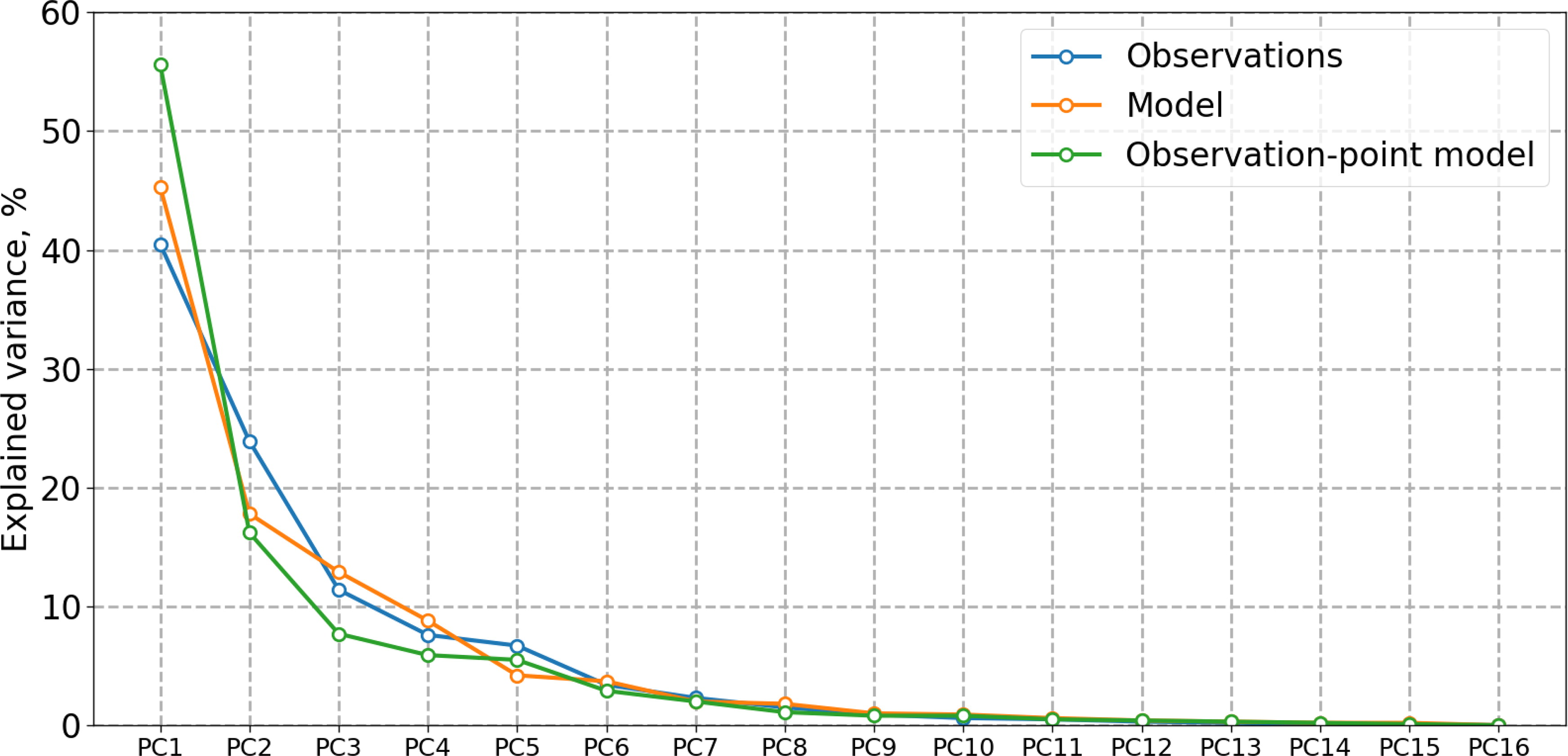
Fig. 3.
Explained percentage of variance of the principal components from all three datasets.
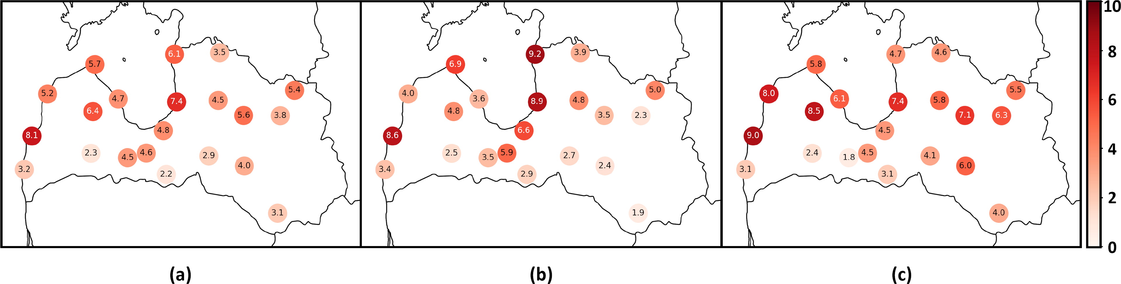
Fig. 4.
EMD (measured in degrees) between observations and model (a) averaged for the whole year, (b) for December and (c) June. Darker (redder) colours indicate higher (worse) EMD values.
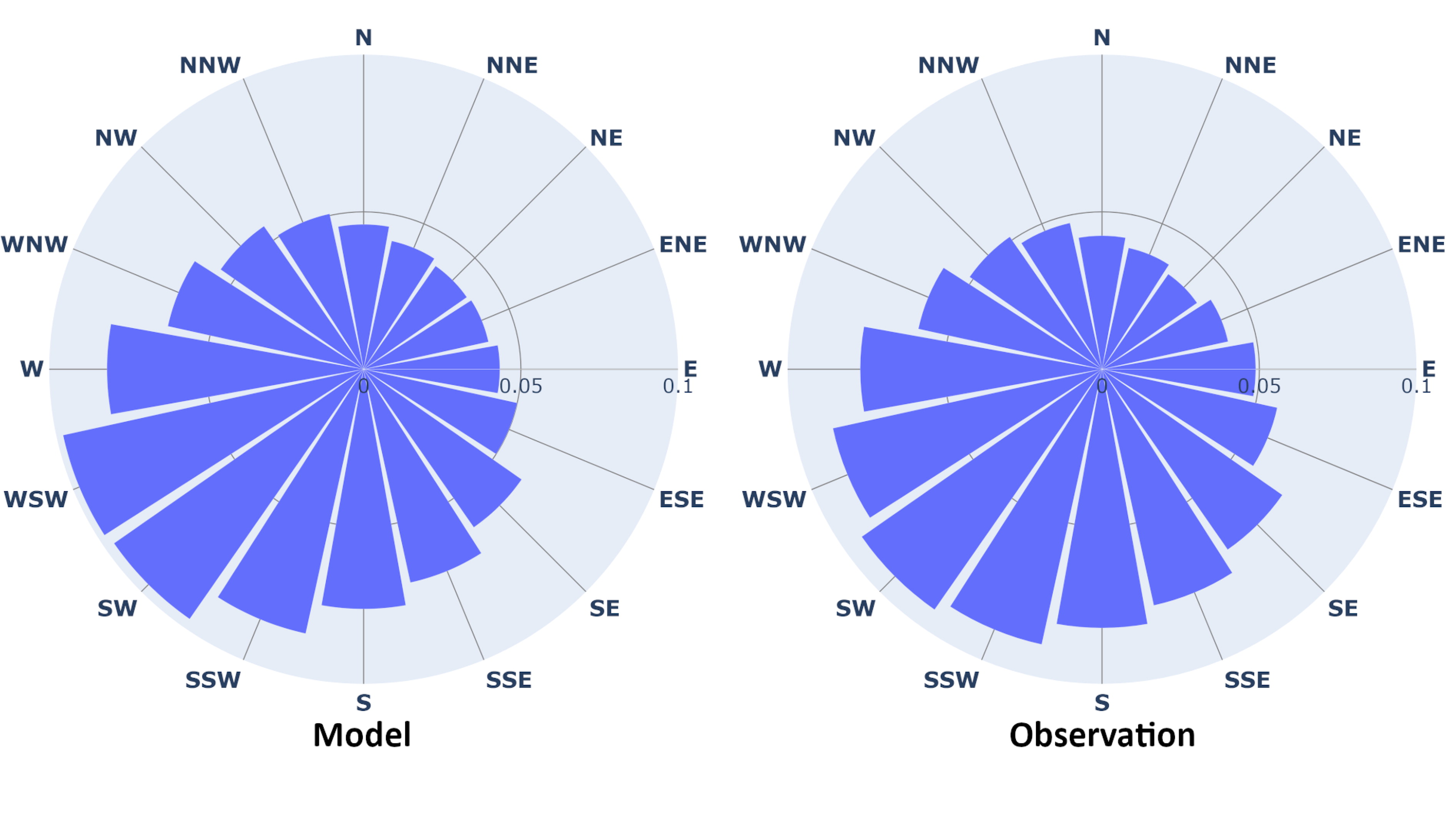
Fig. 5.
Average yearly wind roses for model dataset (left) and observation dataset (right).

Fig. 6.
The loadings of the first 4 principal components for the full model dataset (top row), the observation data (middle row) and the model data from station points only (bottom row). Wind directions are shown on the angular axis, absolute values of the loadings are shown on the radial axis. Grey circles mark increments of 0.1, black circle is at the 0.5 mark. The positive coefficients are red, the negative coefficients are blue. The explained variance of each of the principal components is shown below the loadings.
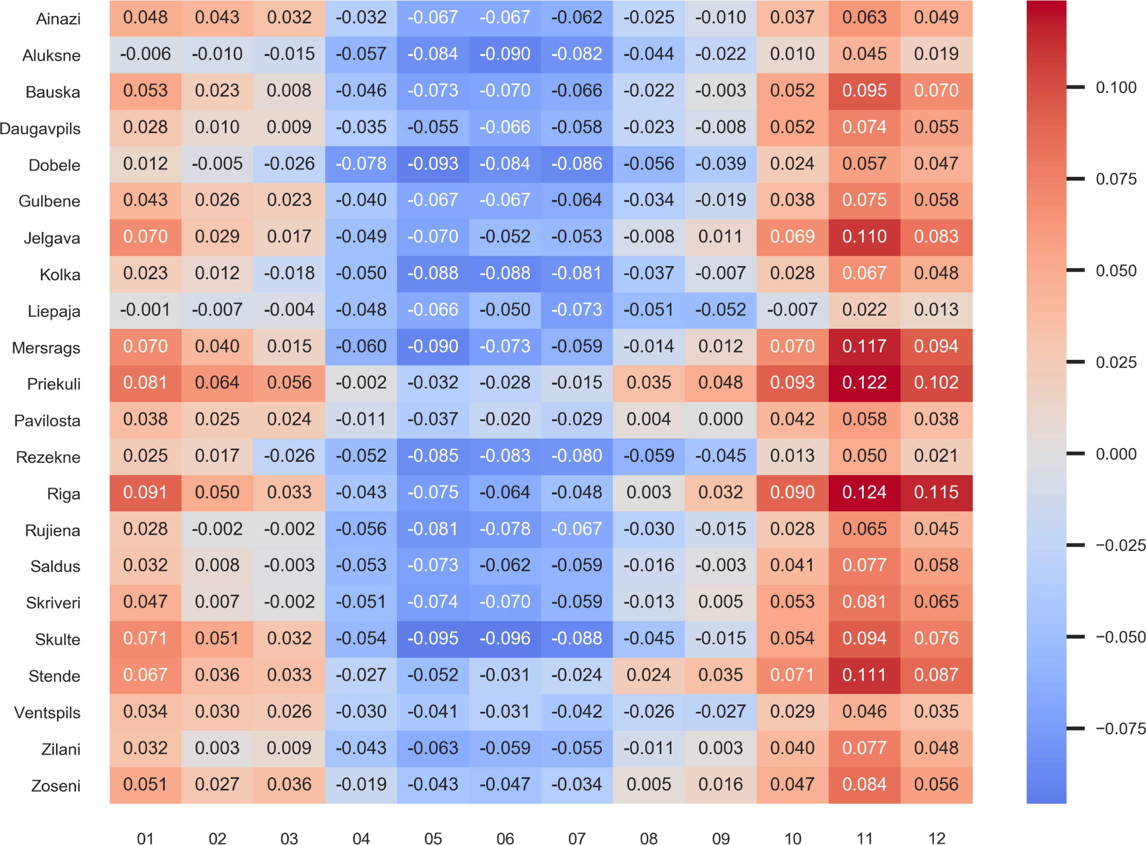
Fig. 7.
Principal component analysis of observation data. Values of PC1 in observation stations (vertical axis) throughout the year. Months are shown on the horizontal axis.
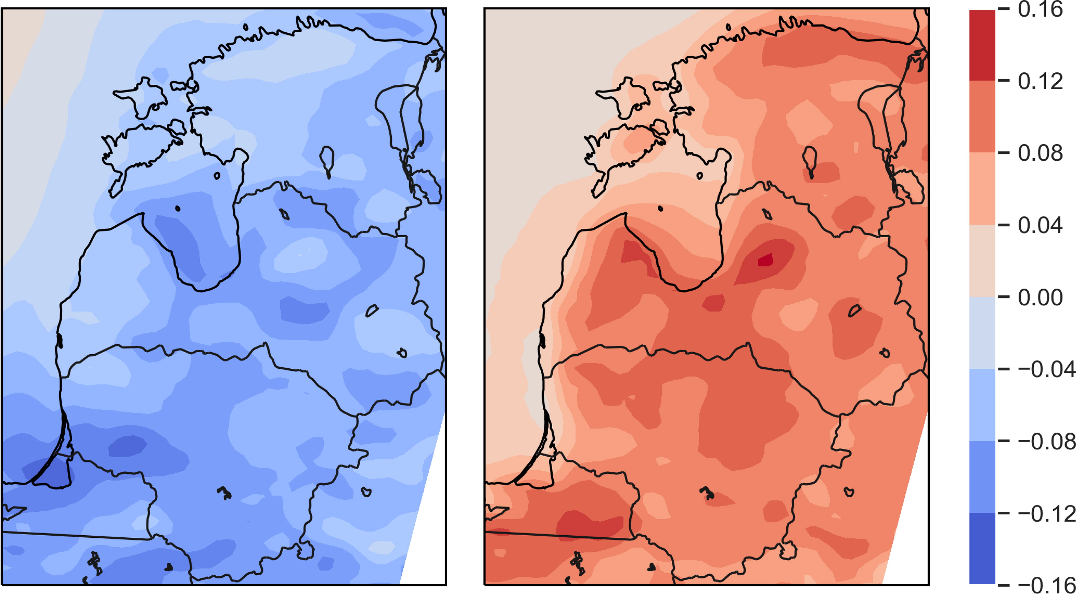
Fig. 8.
Principal component analysis of model data. Values of PC1 in May (left) and November (right).
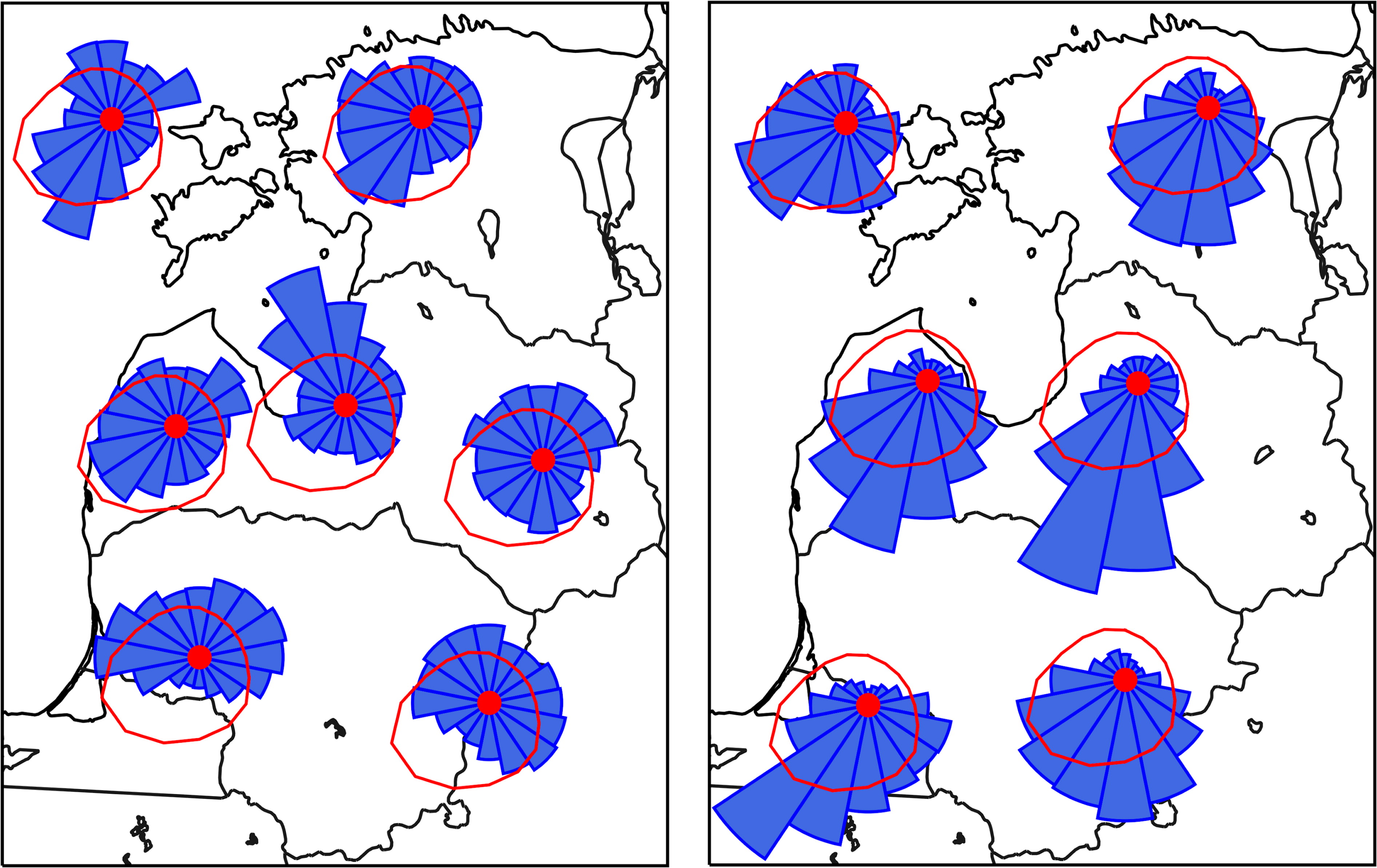
Fig. 9.
Wind direction distribution in model data in May (left) and November (right) at the locations marked by red circles. Average yearly wind rose for the region of study is shown with red line.
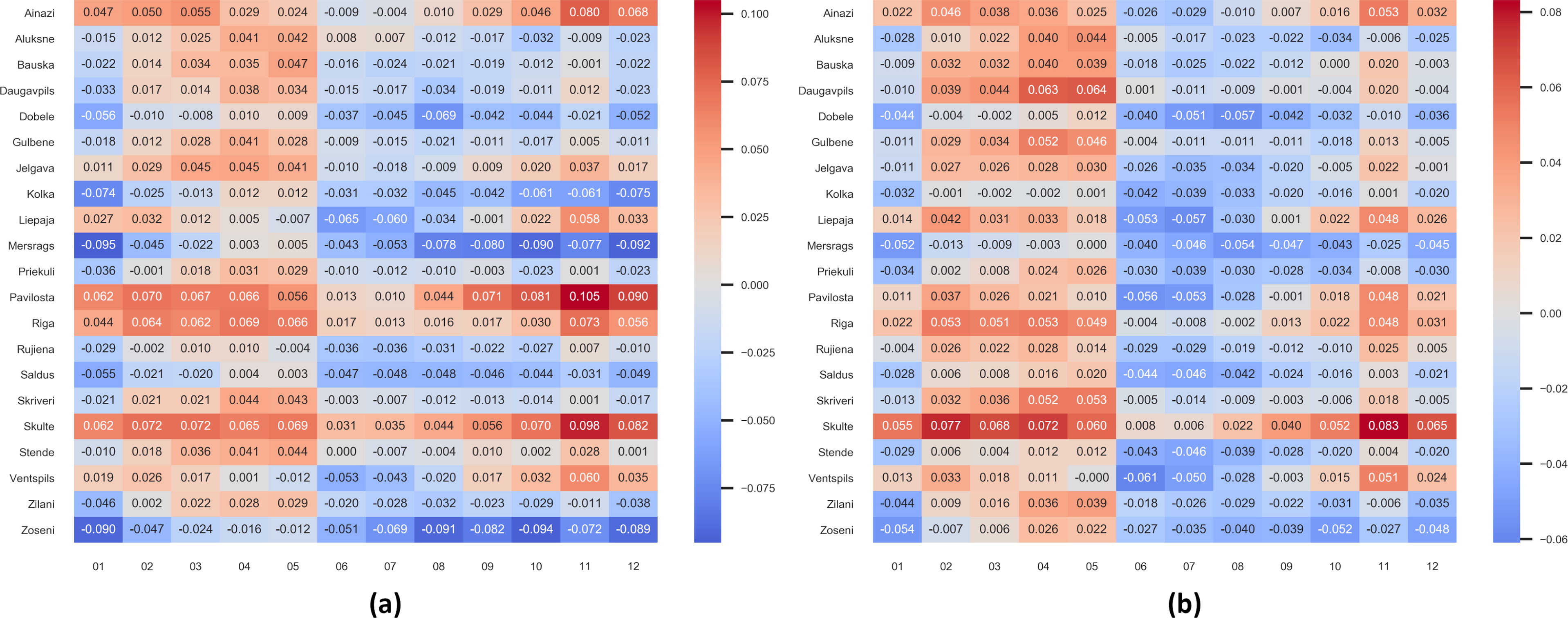
Fig. 10.
Principal component analysis of (a) observation data, (b) model data in observational stations. Values of PC2 of observational data stations (vertical axis) throughout the year. (Months are shown on the horizontal axis.).
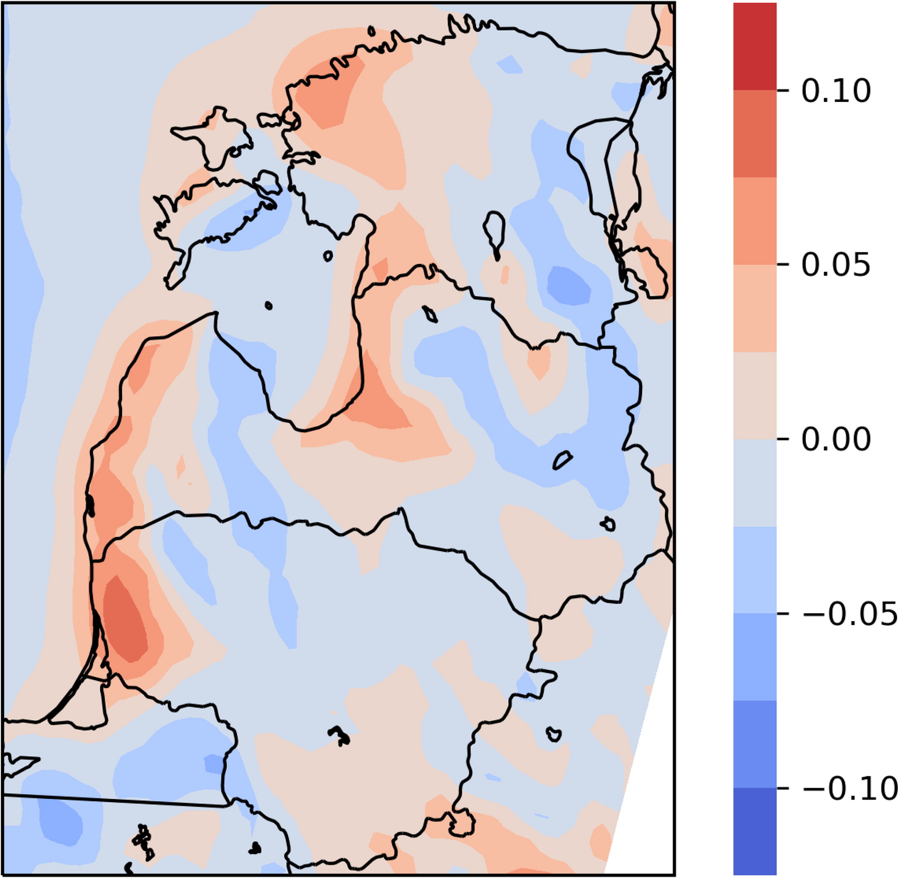
Fig. 11.
Values of PC2 derived from observation data applied to the model data in November.
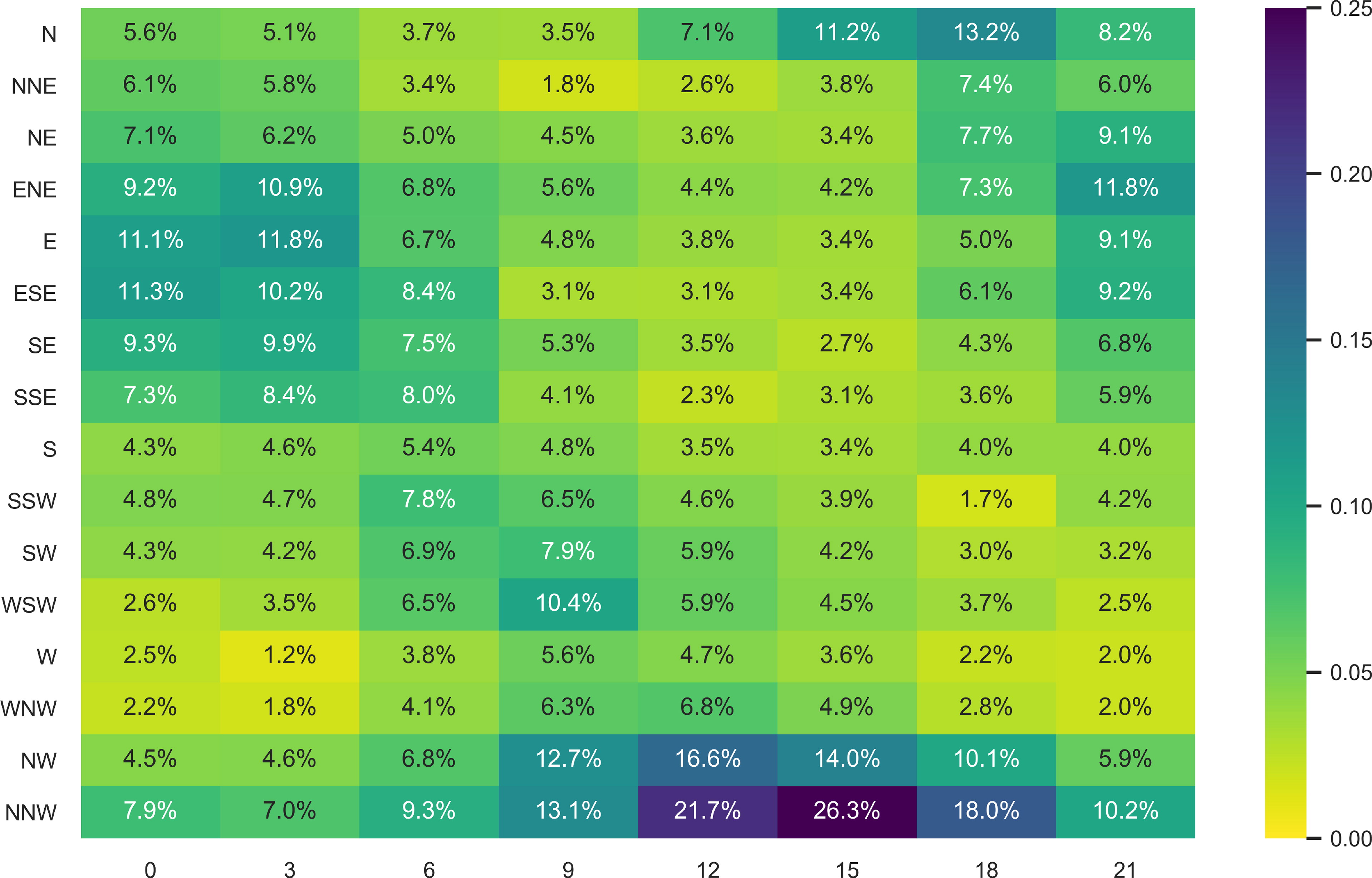
Fig. 12.
Wind direction (y axis) probability distribution (shown with color) at the particular time of the day (x axis, UTC) in Skulte observation station, May, observational data.
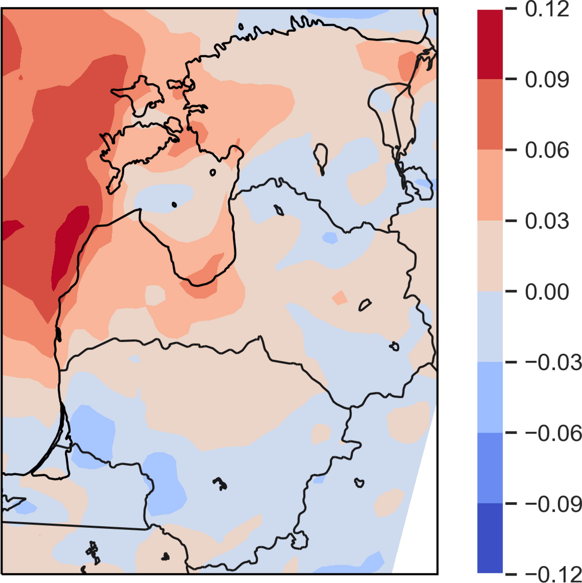
Fig. 13.
Principal component analysis of model data. Values of PC3 in June. The highest values occur over the Baltic sea near the west coast of Latvia.
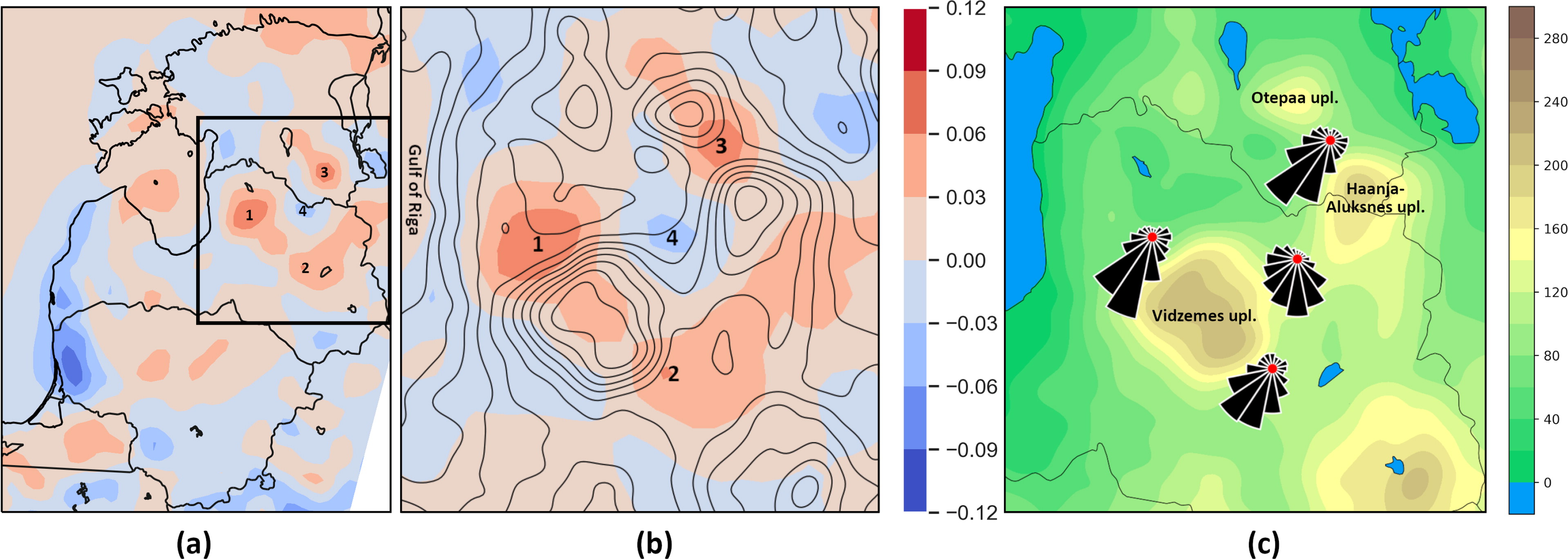
Fig. 14.
(a) Principal component analysis of model data. Values of PC3 in December. (b) Enlarged boxed region from (a). Isolines of altitude (acquired from model data) spaced by 20 metres are shown with black lines. (c) Wind roses for December in points 1-4.