Have a personal or library account? Click to login
Agricultural drought periods analysis by using nonhomogeneous poisson models and regionalization of appropriate model parameters Cover

Agricultural drought periods analysis by using nonhomogeneous poisson models and regionalization of appropriate model parameters

Open Access
|Jan 2021

Figures & Tables

Table 1.

Fitted distributions and methods of parameters estimations.

DistributionParametersMethod of Parameter EstimationNormalσ(scale), µ(location)Method of momentsGammaα(shape), β(scale)Method of momentsGen. Extreme Valueκ(shape), σ(scale), µ(location)Maximum likelihood methodGen. Paretoκ(shape), σ(scale), µ(location)Method of L-momentsPearson-Vα(shape), β(scale), γ(location)Maximum likelihood method
Table 2.

Classification of droughts based on SPI.
SPI valuesSPI Classes2.0 ≤ SPIExtremely wet1.5 ≤ SPI ≤ 1.99Very wet1.0 ≤ SPI ≤ 1.49Moderately wet−0.99 ≤ SPI ≤ 0.99Near normal−1.49 ≤ SPI ≤ −1.0Moderately dry−1.99 ≤ SPI ≤ −1.5Very drySPI ≤ −2.0Extremely dry
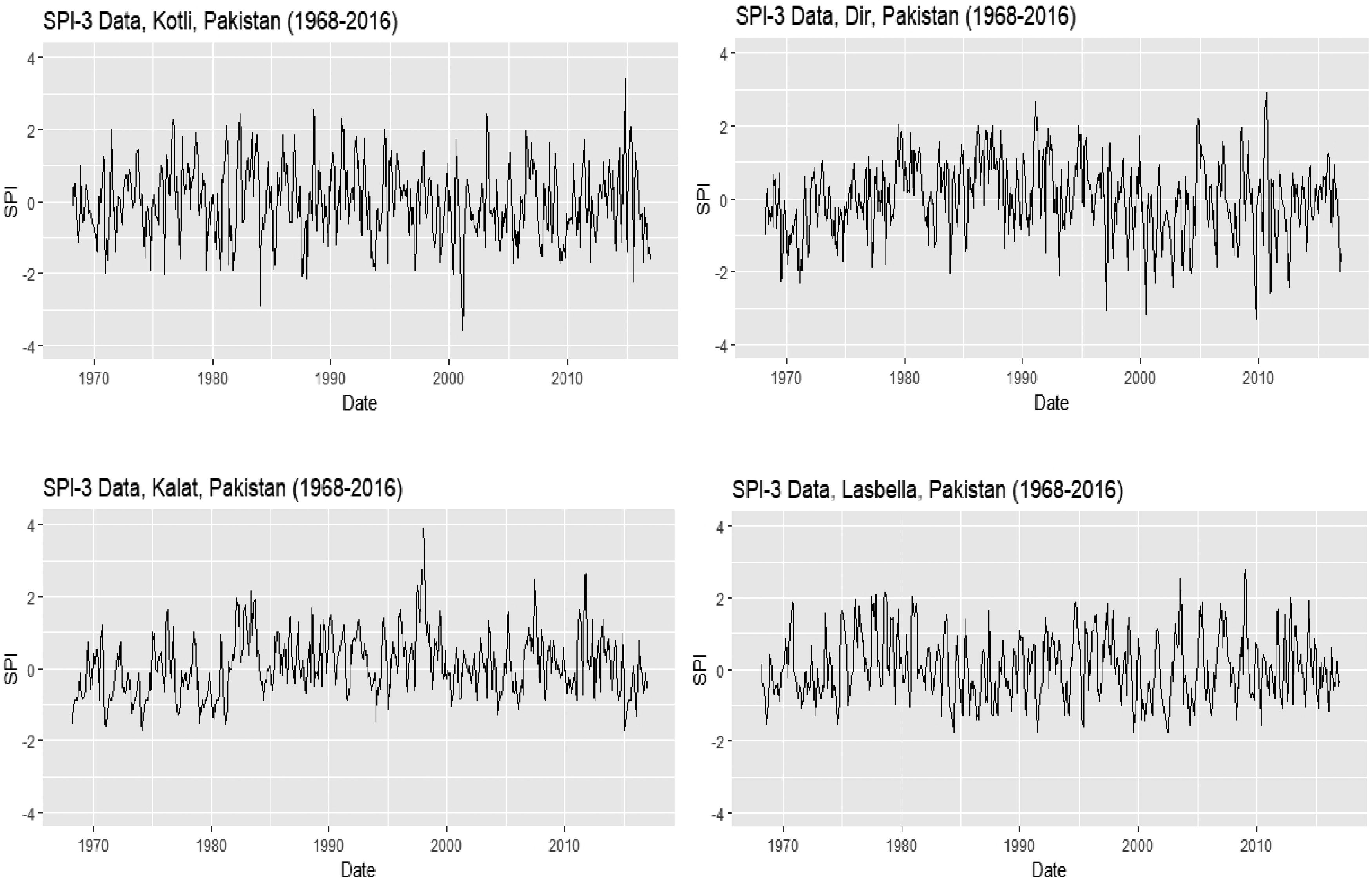
Fig. 1.

The 3-Month standardized precipitation index (SPI −3) versus time (date) (a) Kotli, (b) Dir, (c) Kalat and (d) Lasbella.
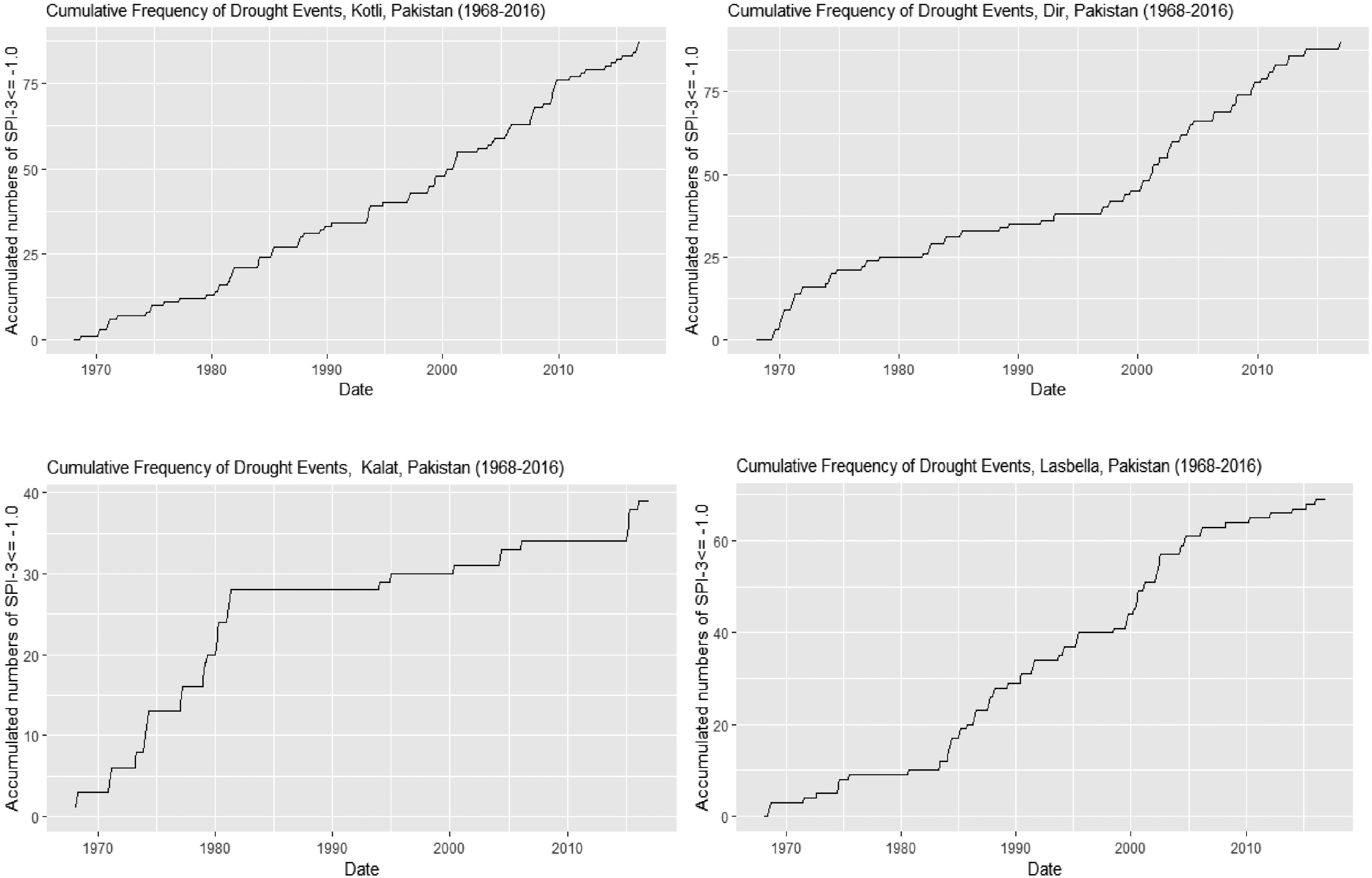
Fig. 2.

Accumulated numbers of SPI − 3 ≤ −1.0 in each time versus month of © (a) Kotli, (b) Dir, (c) Kalat and (d) Lasbella.

Table 3.

Drought periods of each station for 1968-2016 by SPI −3(≤ −1.0).

KotliDirStart dateEnd dateDurationPeakAverageStart dateEnd dateDurationPeakAverage01/09/196801/12/19683−1.13−0.6301/07/196901/07/197124−2.3−1.1801/04/197001/06/19702−1.41−1.3801/11/197101/02/19723−1.58−1.0101/01/197101/06/19715−1.99−1.1201/12/197301/04/197516−1.71−0.7401/11/197101/01/19722−1.42−0.8901/12/197601/01/19771−1.27−1.2701/05/197401/02/19759−1.91−0.7201/04/197701/06/19772−1.87−1.49____________________________________________________________01/07/201501/10/20153−2.23−0.8801/01/201401/03/20142−1.45−1.23LasbellaKalatStart dateEnd dateDurationPeakAverageStart dateEnd dateDurationPeakAverage01/08/196801/12/19684−1.5−0.9601/03/196801/06/196915−1.54−0.8201/08/197101/06/197210−1.08−0.5701/01/197101/12/197111−1.61−0.9301/09/197201/12/19723−1.27−0.7801/04/197301/01/197521−1.73−0.901/07/197401/12/19745−1.53−0.9601/02/197701/04/197814−1.27−0.5601/07/197501/01/19766−1.02−0.4901/01/197901/10/198021−1.53−0.94____________________________________________________________01/02/201601/05/20163−1.15−0.4601/02/201601/04/20162−1.34−0.67
Table 4.

List of the total number of agricultural droughts at each station (1968-2016).
StationsTotal EventsStationsTotal EventsStationsTotal EventsStationsTotal EventsCherat80Lasbella69Padidan66Sargodha98Peshawar94Zohub92Rohri24Murree94Kakul108Nokkundi24Badin33Mianwali88DIK82Khuzdar81Chhor28Bahawalnagar80Drosh97Barkhan70Karachi69Gilgit91Parachinar81Faisalabad93Nawabshah50Sakardu86Kohat102Jhelum101Dalbadin39Bunji98Risalpur90Sialkot87Panjgur42Chilas84Balakot95BahawalPur79Pasni33Astore95Chitral100Multan83Kalat39Gupis73Dir90Khanpur53Quetta56Kotli87Hyderabad44Lahore89Sibbi63Muzafarabad88Jacobabad63Rawalpindi98Jiwani22Garhi Dupatta92
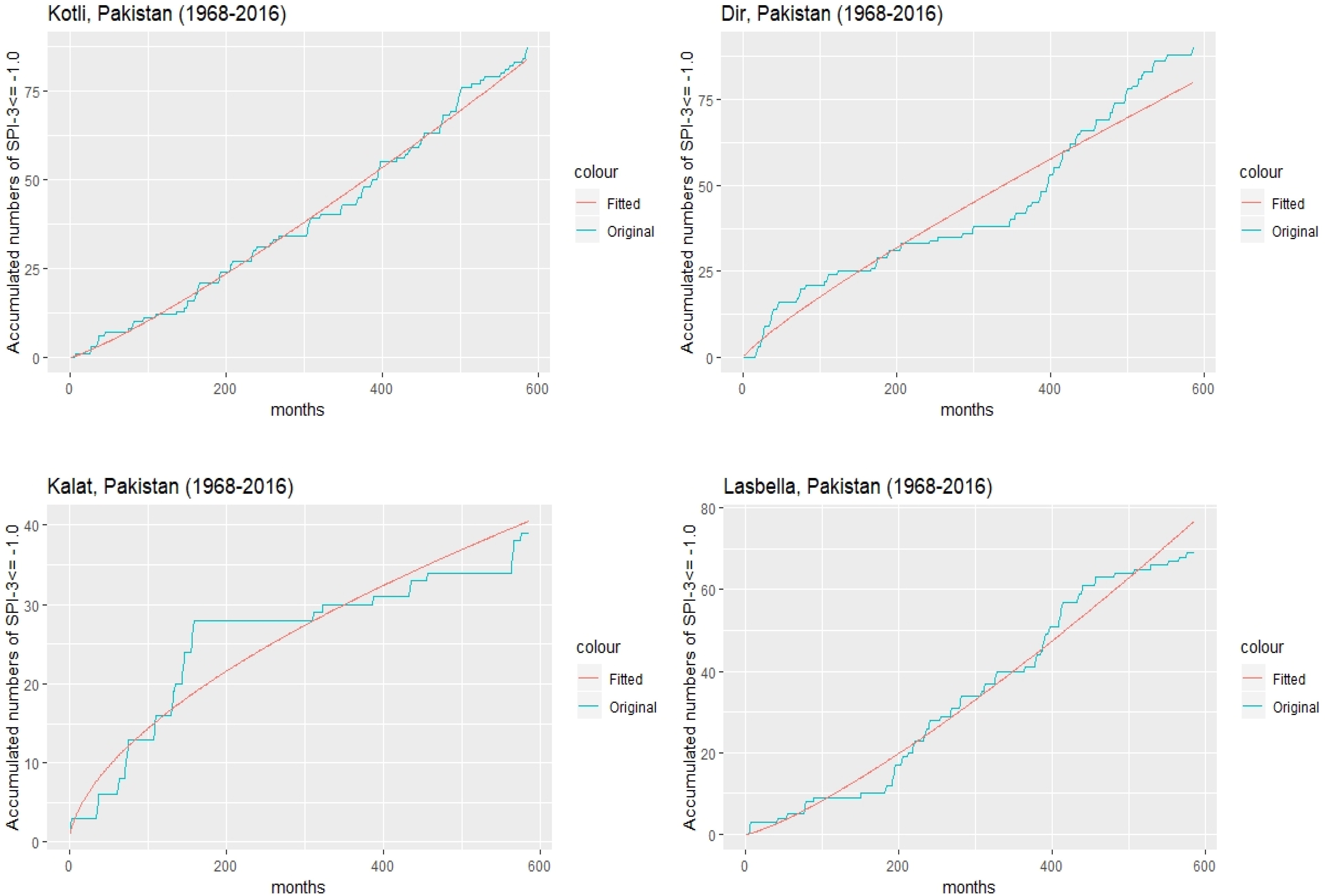
Fig. 3.

Plots of Accumulated numbers of SPI −3 ≤ −1.0 in each time with the estimated mean value function versus month of ©. (a) Kotli, (b) Jiwani, (c) Mianwali, and (d) Barkhan.

Table 5.

Values of DIC for power-law process and linear intensity function models.

ModelsDICLinear Intensity Function189044Power Law Process173266
Table 6.

RMSEs of each station for observed vs estimated accumulated drought events.
StationsRMSEStationsRMSEStationsRMSECherat2.8630Nawabshah3.1398Khanpur1.7831Peshawar2.8028Dalbadin3.8555Lahore4.8889Kakul5.8521Panjgur3.5737Rawalpindi2.4249DIK3.2788Pasni2.0577Sargodha2.7688Drosh2.4722Kalat3.4705Murree6.8652Parachinar4.1849Quetta4.2837Mianwali5.6827Kohat4.5213Sibbi4.6927Bahawalnagar3.5966Risalpur2.9361Jiwani1.5600Gilgit4.4050Balakot4.1720Lasbella3.4502Sakardu2.1707Chitral3.2353Zohub3.1586Bunji3.2027Dir6.5661Nokkundi1.2927Chilas6.3755Hyderabad2.6348Khuzdar3.4265Astore4.0773Jacobabad3.3215Barkhan4.9927Gupis8.4248Padidan3.7135Faisalabad4.2647Kotli2.1358Rohri0.9458Jhelum2.6521Muzaffarabad3.8791Badin1.8745Sialkot3.7204GarhiDupatta3.7050Chhor1.9242BahawalPur5.4079Karachi2.5290Multan2.1890
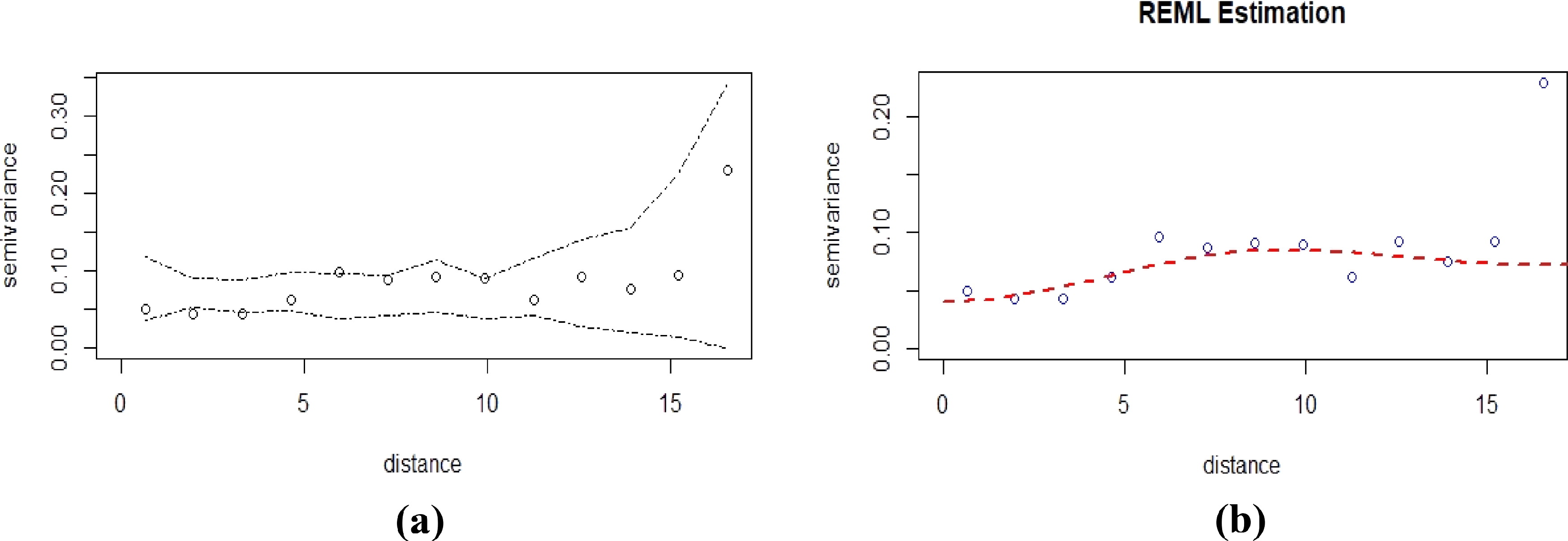
Fig. 4.

Observed variogram, variogram envelope, and fitted variogram for α.

Table 7.

Parameters and RMSE's of variogram models in case of α.
MethodsModelsNuggetSillRangeRMSEMethodsModelsNuggetSillRangeRMSEMLMetern0.03110.05195.48650.201258OLSMetern0.032732.69765313.9040.19324Spherical0.03310.042710.26130.199141Spherical0.032815.4093769.4070.19326Cubic0.03310.0365.36480.208773Cubic0.0491157.1931722.9010.22421Exponential0.03110.05195.48650.201258Exponential0.032732.69765313.9040.19324Cauchy0.03970.0451454.3290.197553Cauchy0.0492268.05602.67320.22515Wave0.04010.02772.02210.20096Wave0.049164.4585170.62280.22516REMLMetern0.03132.2563295.2870.192497WLSMetern0.02490.07686.11630.19979Spherical0.03190.052410.55210.198267Spherical0.0240.06269.20550.20142Cubic0.03290.04135.62930.208115Cubic0.03310.054411.16780.20452Exponential0.03132.2563295.2870.192497Exponential0.02490.07686.11630.19979Cauchy0.0390.20228.05180.199316Cauchy0.03550.08063.76880.19907Wave0.04010.03682.12370.192013Wave0.03270.04721.82210.21026
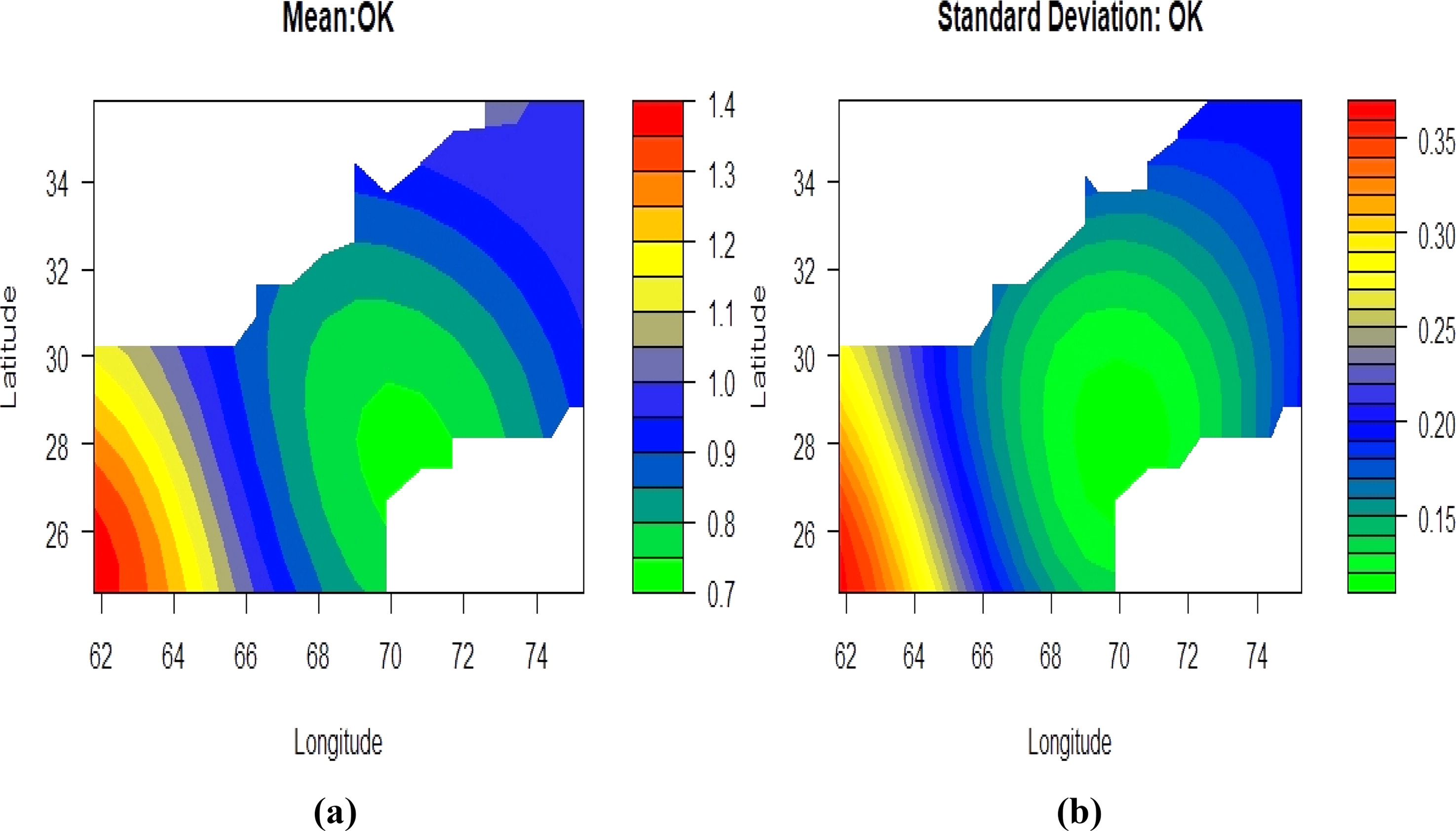
Fig. 5.

Spatial interpolation and associated prediction error for parameter α.
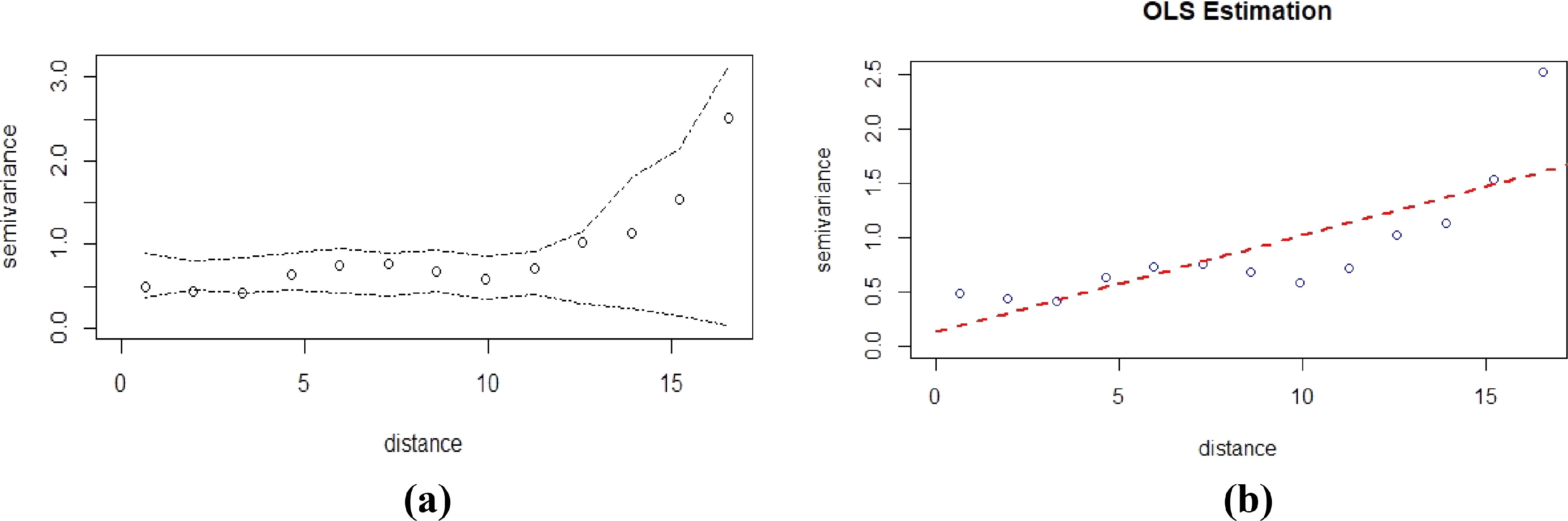
Fig. 6.

Observed variogram, variogram envelope, and fitted variogram for β.

Table 8.

Parameters and RMSE's of variogram models in case of β.
MethodsModelsNuggetSillRangeRMSEMethodsModelsNuggetSillRangeRMSEMLMetern0.32490.43586.688913.0437OLSMetern0.132211658130663.68.63995Spherical0.33650.341110.588113.1787Spherical0.1327783.905213187.998.6436Cubic0.38150.338613.947512.5888Cubic0.34914179.7812284.16814.6308Exponential0.32490.43586.68913.0437Exponential0.13265841.62765506.278.6433Cauchy0.38670.3574377.52612.3193Cauchy0.35063126.162529.867314.7507Wave0.38060.35415.831714.7532Wave0.35909.1843164.873414.7566REMLMetern0.325221.6513400.66910.4671WLSMetern0.35691185.48526079.7910.9931Spherical0.32518.8044245.0110.4208Spherical0.3573118.75853925.58310.9984Cubic0.38060.553316.820110.7795Cubic0.46511780.0371934.11414.7747Exponential0.325222.7968422.03610.4655Exponential0.35691303.16828669.3610.9931Cauchy0.38041.43527.91510.0929Cauchy0.46571422.229463.786214.8388Wave0.39870.34862.432111.7545Wave0.4655440.6046149.021714.8421
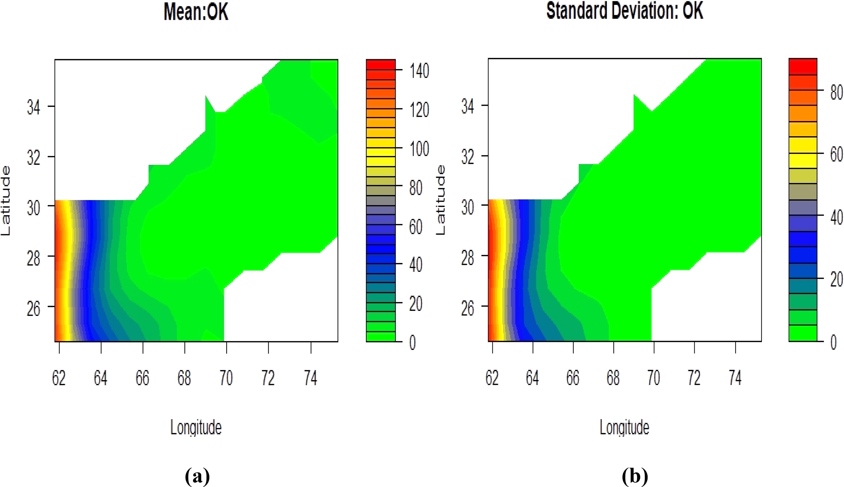
Fig. 7.

Spatial interpolation and associated prediction error for parameter β.

Language: English
Page range: 1948241 - 1948241
Published on: Jan 1, 2021
Published by: Stockholm University Press
In partnership with: Paradigm Publishing Services

© 2021 Asad Ellahi, Ijaz Hussain, Muhammad Zaffar Hashmi, Mohammed Mohammed Ahmed Almazah, Fuad S. Al-Duais, published by Stockholm University Press
This work is licensed under the Creative Commons Attribution 4.0 License.