
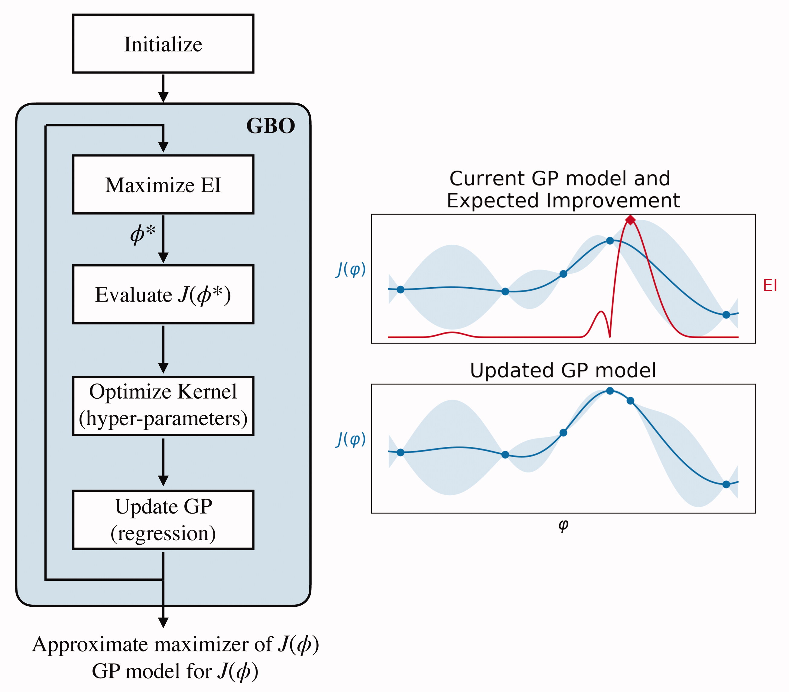
Fig. 1.
Flowchart of the GBO algorithm. The two panels on the right illustrate (i) how maximization of expected improvement results in additional function evaluations that explore the space effectively; and (ii) the effects of a typical update of the GP mean and covariance based on a single, additional function evaluation.
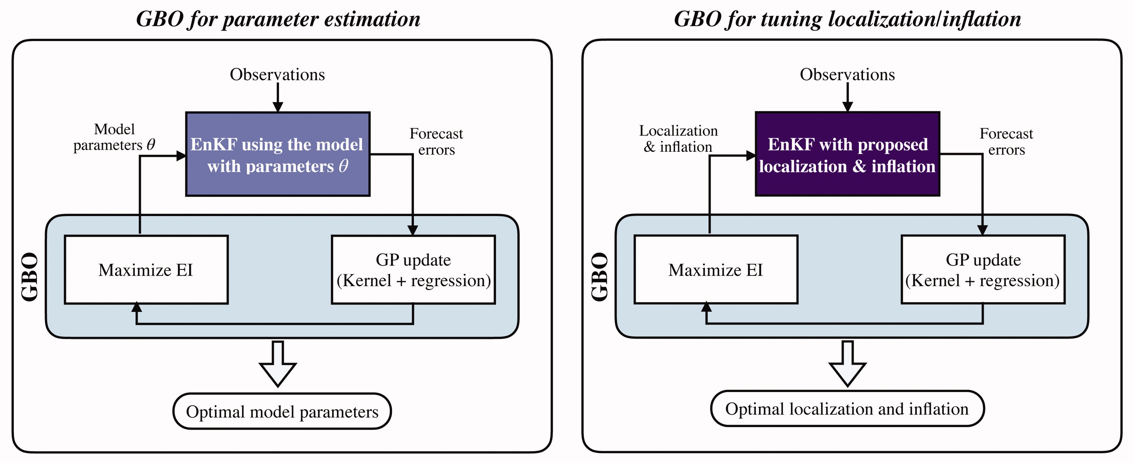
Fig. 2.
Flowchart of the GBO used for parameter estimation (left) and tuning of localization/inflation (right). Note that the algorithms are essentially the same for both tasks, and differ only in the parameters being handed back and forth between the ensemble DA (EnKF) and the GBO iterations. We highlight this difference by using different colors for the parameter estimation (blue) and the tuning of localization/inflation (purple).
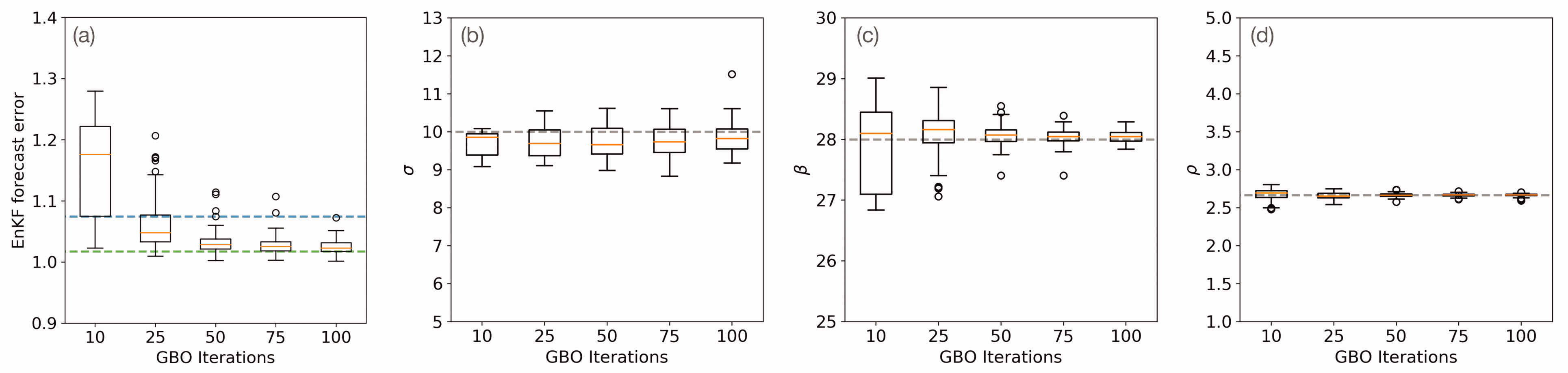
Fig. 3.
Summary of results for the parameter estimation of Lorenz ’63. (a) Box-and-whisker plot of time averaged forecast RMSE. Dashed blue: RMSE of the augmented state EnKF. Dashed green: RMSE of an EnKF using the ‘true’ model parameters. Statistical variation of RMSE for the EnKF or augmented state EnKF is too small to be visible on the scale of the plot. (b)–(d) Box-and-whisker plots of the model parameters σ, β and ρ. The limits of the y-axes in (b)–(d) are set to reflect the assumed bounds on the model parameters. In each box-and-whisker plot, the orange line is the median, the box spans the first and third quartiles, the whiskers are the minimum/maximum and dots represent outliers (if applicable).
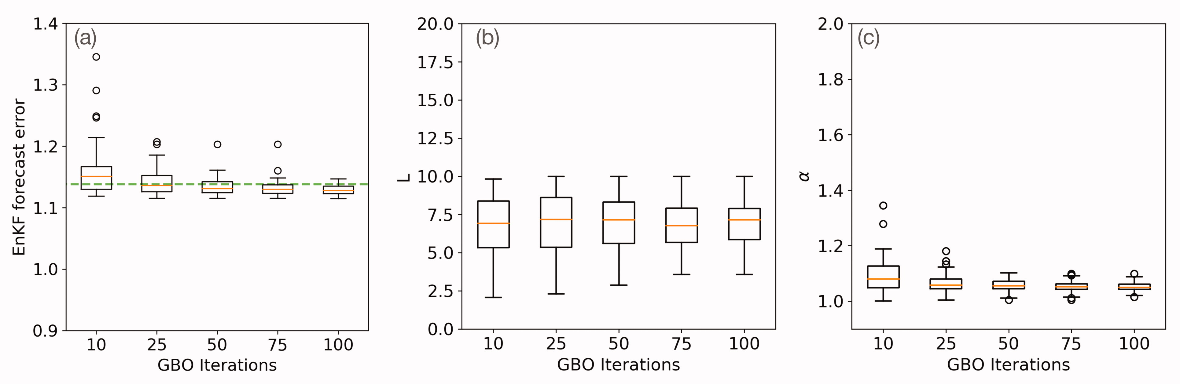
Fig. 4.
Summary of results for tuning localization and inflation in Lorenz ’96. (a) Box-and-whisker plot of time averaged forecast RMSE. Dashed green: time-averaged forecast RMSE of an EnKF with localization/inflation tuned by a grid-search (statistical variation of RMSE is too small to be visible on the scale of the plot). (b) and (c) show box-and-whisker plots of localization (L) and inflation (α) parameters as a function of GBO iterations. The limits of the y-axes in (b) and (c) are set to reflect the assumed bounds on the localization/inflation parameters. In each box-and-whisker plot, the orange line is the median, the box spans the first and third quartiles, the whiskers are the minimum/maximum and dots represent outliers (if applicable).
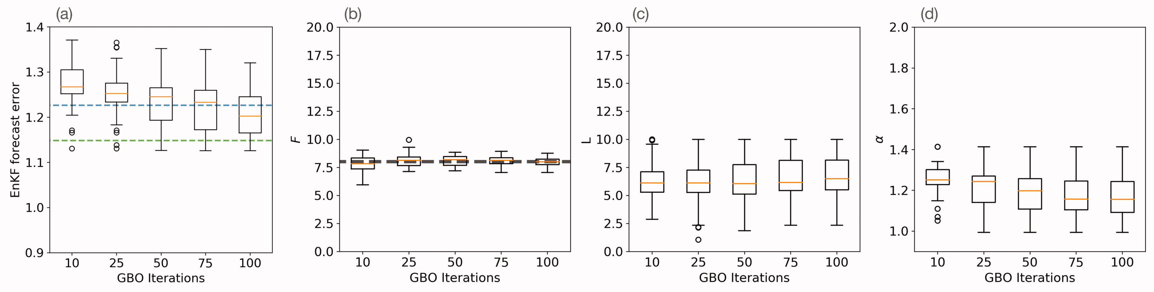
Fig. 5.
Summary of results for tuning localization and inflation while estimating a model parameter in Lorenz ’96. (a) Box-and-whisker plot of time averaged forecast RMSE. Dashed blue: RMSE of the augmented state EnKF. Dashed green: RMSE of an EnKF using the ‘true’ model parameters. Statistical variation of RMSE for the EnKF or augmented state EnKF is too small to be visible on the scale of the plot. (b)–(d) show box-and-whisker plots of the forcing F, localization (L) and inflation (α) parameters as a function of GBO iterations. The limits of the y-axes in (b)–(d) are set to reflect the assumed bounds on the model and localization/inflation parameters. In each box-and-whisker plot, the orange line is the median, the box spans the first and third quartiles, the whiskers are the minimum/maximum and dots represent outliers (if applicable).