
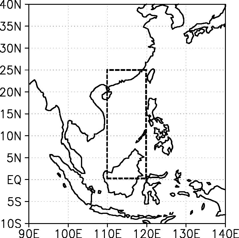
Fig. 1.
Definition of South China Sea (SCS) domain (0°-25°N, 110°E-120°E) in this study.
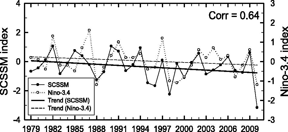
Fig. 2.
Time series of South China Sea summer monsoon (SCSSM) index and Niño-3.4 index and their trends for June-September (JJAS). Even though the decreasing trend of the Niño-3.4 index is insignificant, the decreasing trend of the SCSSM index is significant at the 90% confidence level.
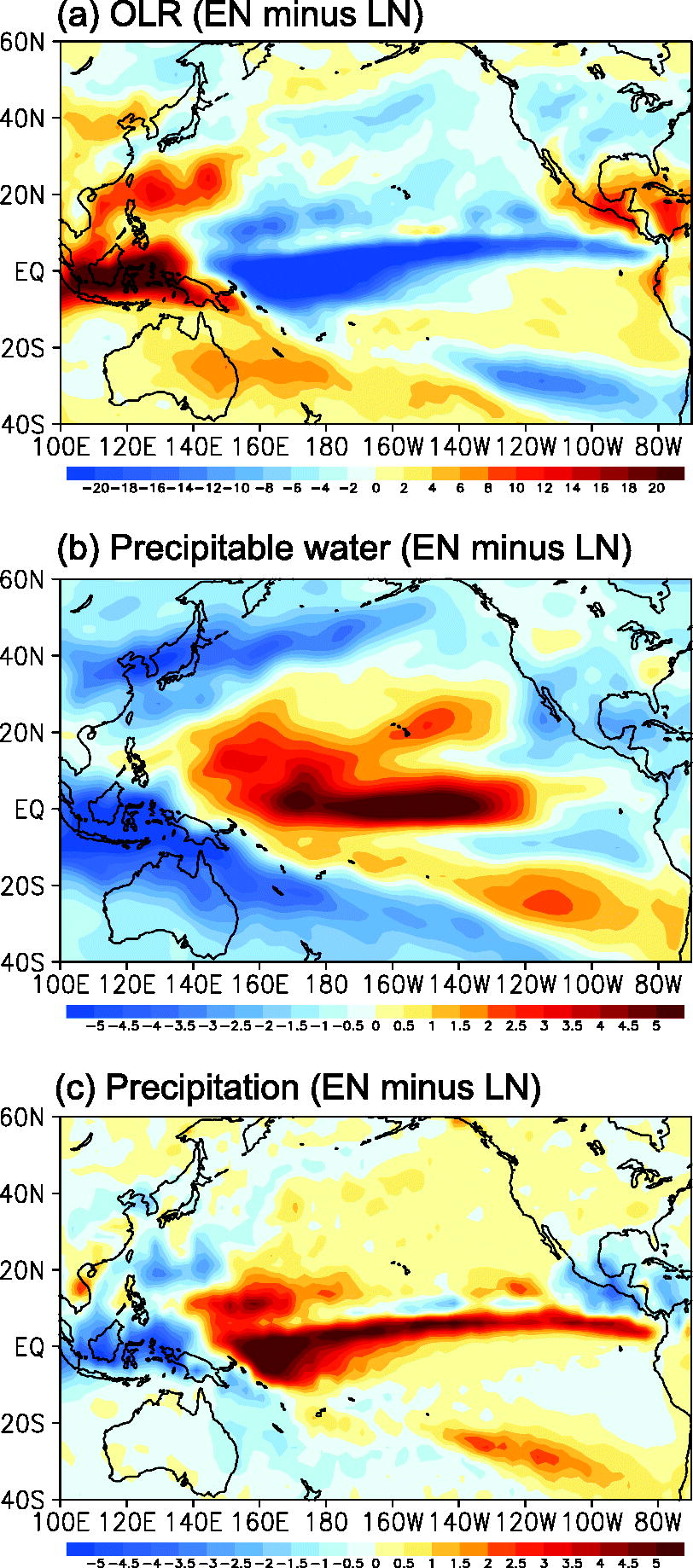
Fig. 3.
Differences in (a) OLR, (b) precipitable water, and (c) precipitation between El Niño years and La Niña years.

Fig. 4.
Same as in Fig. 3, but for (a) 850 hPa stream flows and (b) 200 hPa stream flows. Shaded areas are significant at the 95% confidence level.
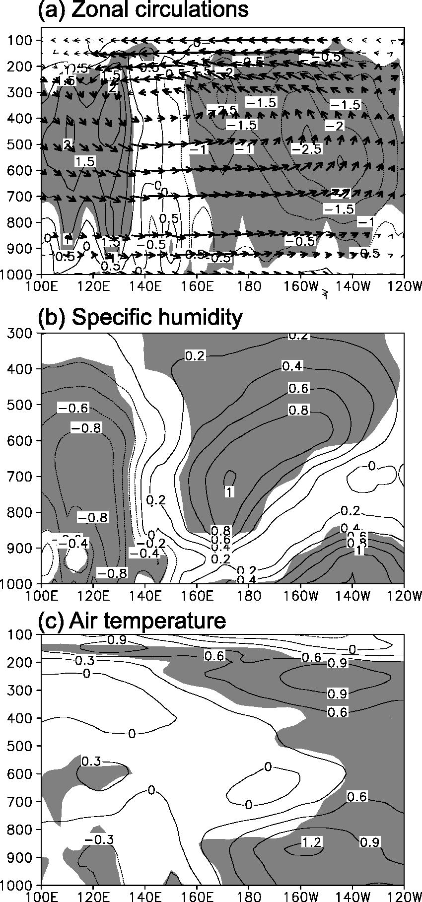
Fig. 5.
Composite differences of longitude–pressure cross section of (a) vertical velocity (contours) and zonal circulations (vectors), (b) specific humidity, and (c) air temperature averaged along 0°-20°N between El Niño years and La Niña years for JJAS. The values of vertical velocity are multiplied by −100. Bold arrows and shaded areas are significant at the 90% confidence level. Contour intervals are 0.5−2hPa s−1 for vertical velocity, 0.2 g kg−1 for specific humidity, and 0.3 °C for air temperature, respectively.
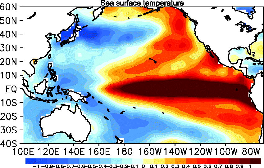
Fig. 6.
Same as in Fig. 3, but for sea surface temperature (SST).
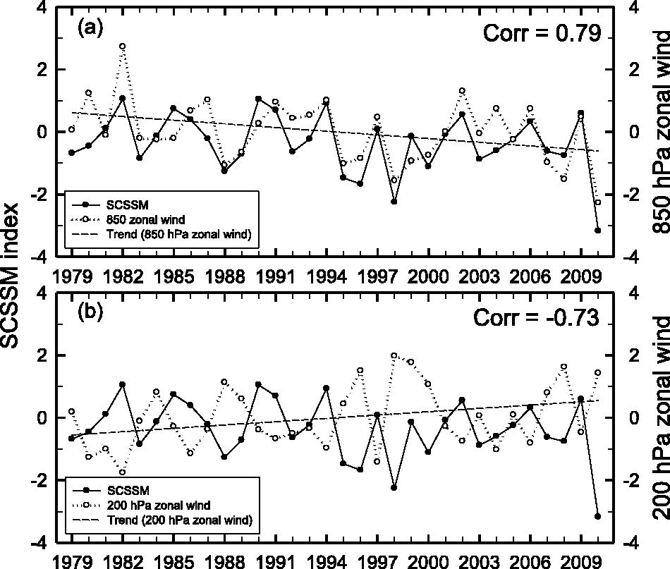
Fig. 7.
Time series of SCSSM index and (a) 850 hPa zonal wind and (b) 200 hPa zonal wind averaged for Niño-3.4 region (5°S-5°N, 170°E-120°W). The trends of 850 hPa zonal wind and 200 hPa zonal wind are significant at the 90% and 95% confidence levels, respectively.

Fig. 8.
Differences in the mean TC passage frequencies between El Niño years and La Niña years for JJAS within each 5°×5° latitude-longitude grid box. Small solid rectangles indicate that the differences are significant at the 95% confidence level.
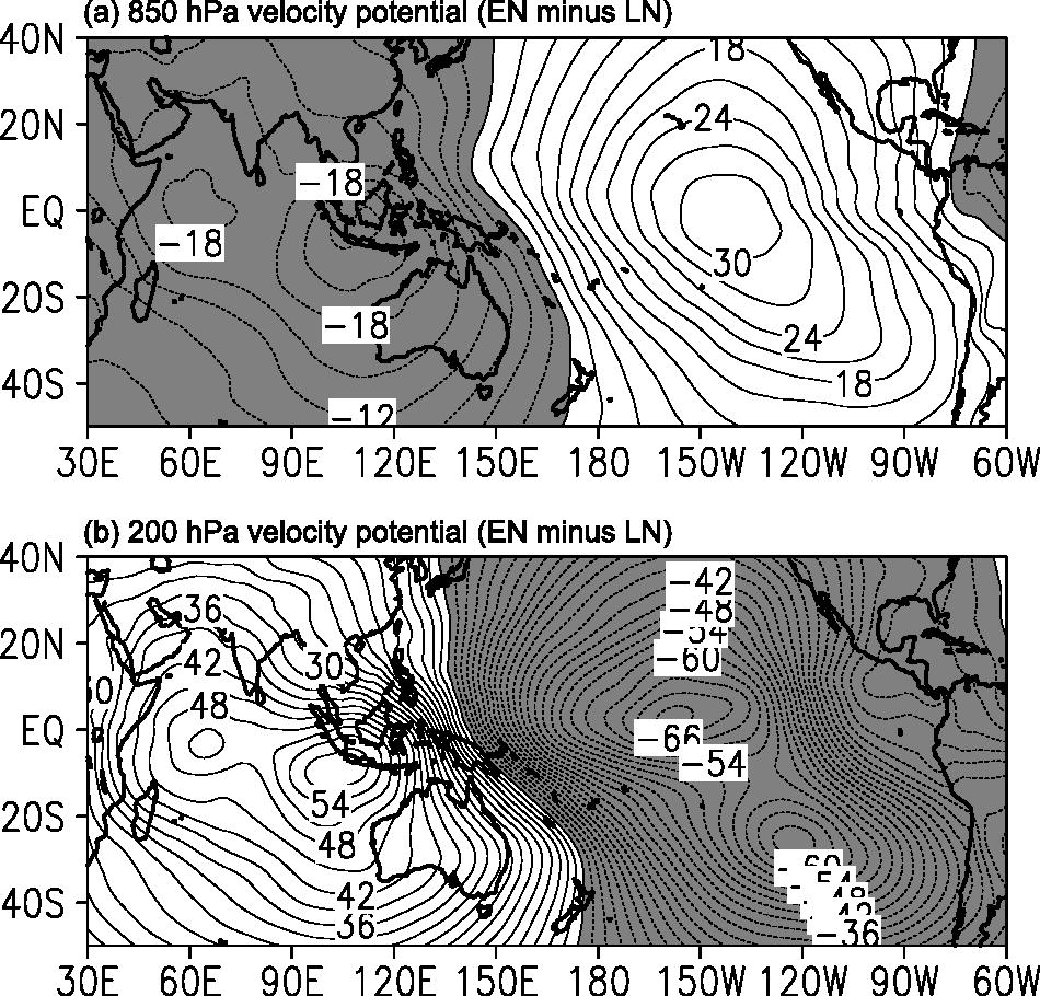
Fig. 9.
Same as in Fig. 3, but for (a) 850 hPa velocity potential and (b) 200 hPa velocity potential. Shaded areas denote negative anomalies. Contour interval is 3 m2s−110−6.