
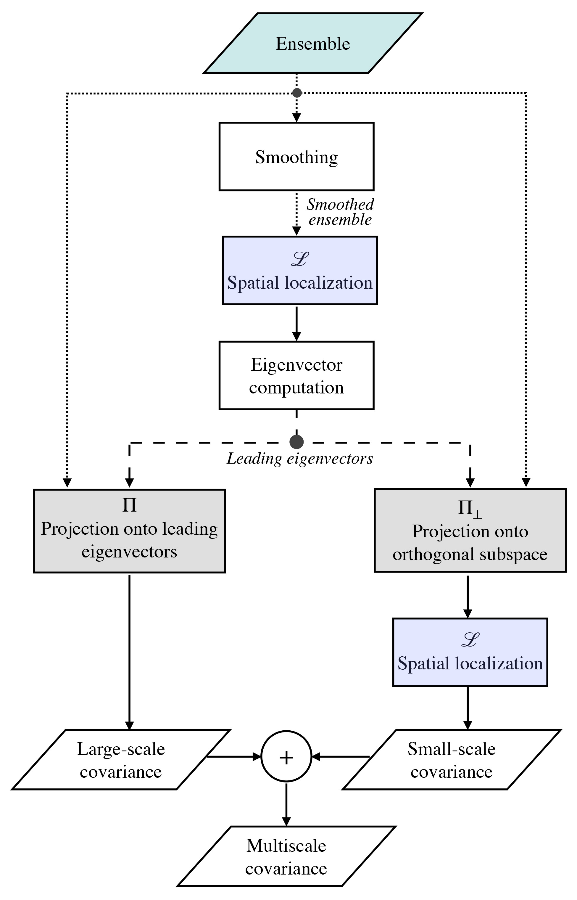
Fig. 1.
Flowchart of ESL. Rounded boxes are operations and trapezoids are inputs and outputs (some intermediate inputs and outputs are omitted for clarity). Dotted lines represent ensembles, solid lines represent covariance matrices, and dashed lines represent a collection of eigenvectors.
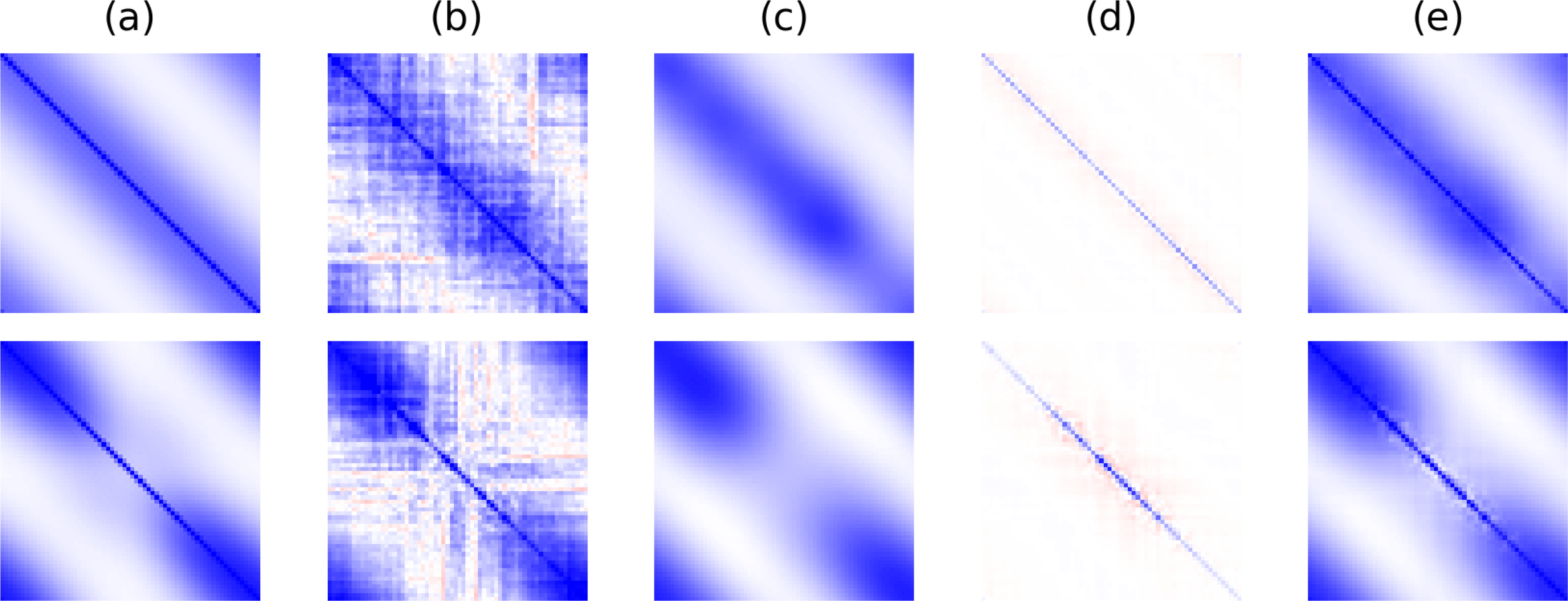
Fig. 2.
Illustration of the homogeneous (top row) and heterogeneous (bottom row) systems (see also the numerical illustrations in Section 4). The colour indicates the value of the elements of a covariance matrix after being clipped between -1 and 1, where blue shades are positive and red shades are negative. Column (a): true covariance matrix Column (b): sample covariance matrix of an ensemble of size 40. Column (c): large-scale covariance matrix (Section 3.1). Column (d): small-scale covariance matrix (Section 3.2). Column (e): multiscale covariance matrix
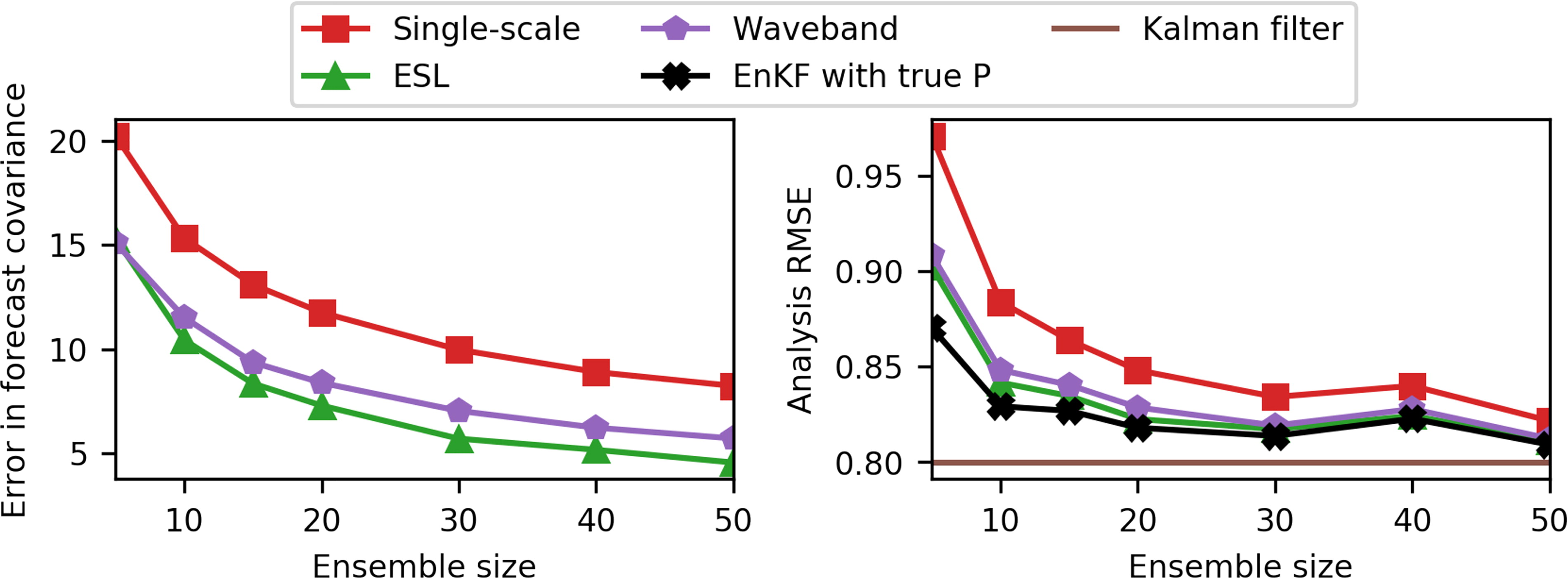
Fig. 3.
Results for the case of an isotropic homogeneous forecast covariance. Left: Error in forecast covariance matrix (Frobenius norm) as a function of ensemble size. Right: Analysis RMSE as a function of ensemble size. Green triangles: ESL. Purple hexagons: waveband localisation. Red squares: single-scale localisation. Black x’s (right panel): EnKF using true forecast covariance. Brown line (right panel): average analysis standard deviation of the Kalman filter.
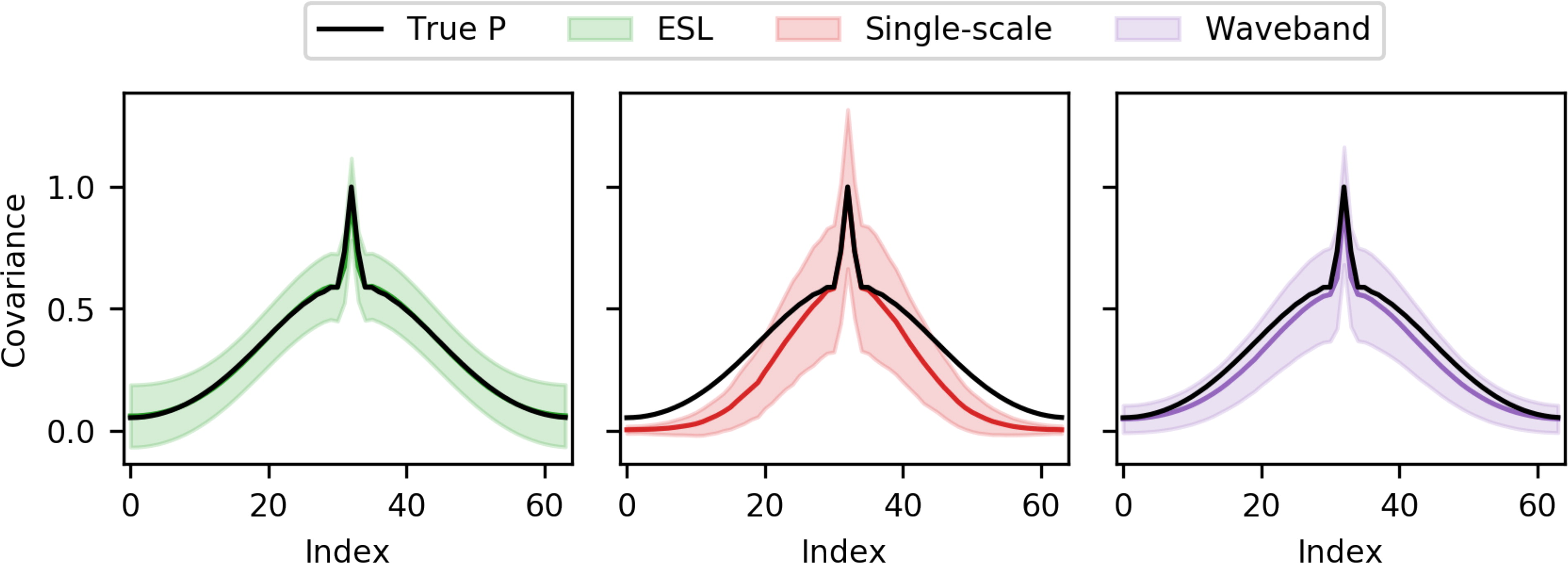
Fig. 4.
Results for the case of an isotropic homogeneous forecast covariance. Shown is the covariance with index 32, which falls roughly in the centre of the domain. Left (green): ESL. Centre (red): single-scale localisation. Right (purple): Waveband localisation. The solid lines show the covariance averaged over 1000 trials, and the shaded region shows this average plus and minus one standard deviation. In all three panels, the true covariance is shown with a solid black line.
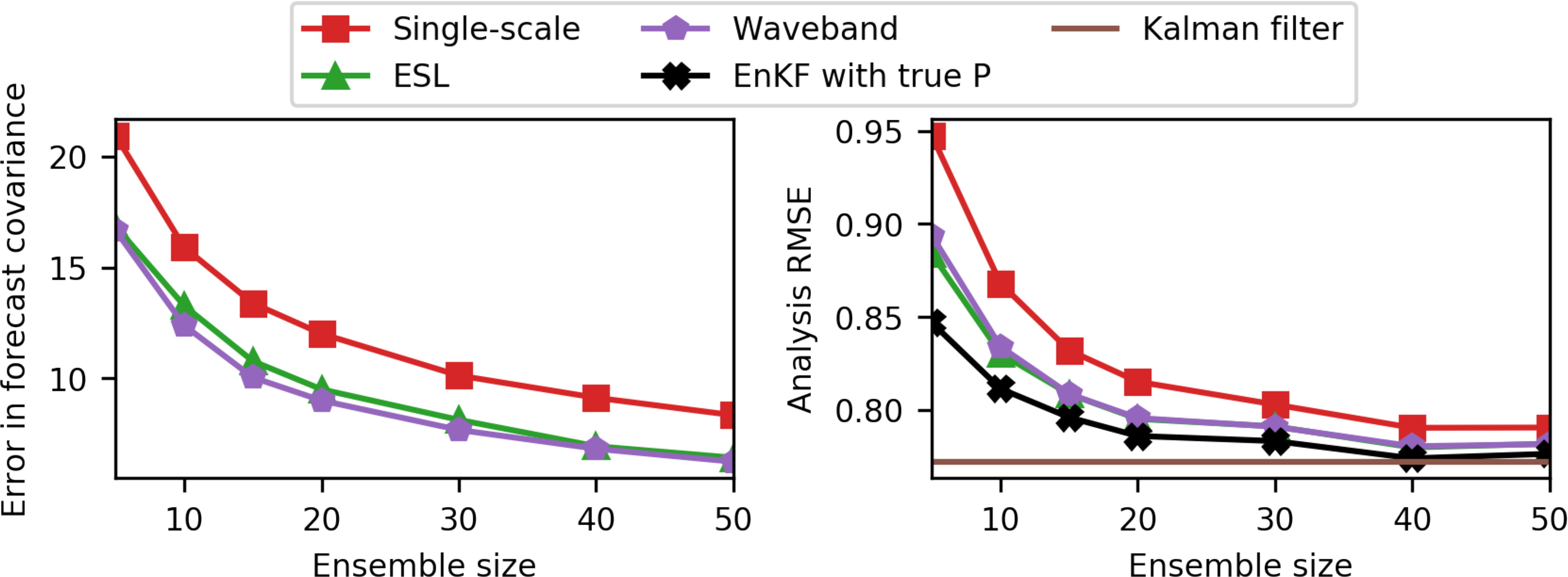
Fig. 5.
Results for the case of a heterogeneous forecast covariance. Left: Error in forecast covariance matrix (Frobenius norm) as a function of ensemble size. Right: Analysis RMSE as a function of ensemble size. Green triangles: ESL. Purple hexagons: waveband localisation. Red squares: single-scale localisation. Black x’s (right panel): EnKF using true forecast covariance. Brown line (right panel): average analysis standard deviation of the Kalman filter.
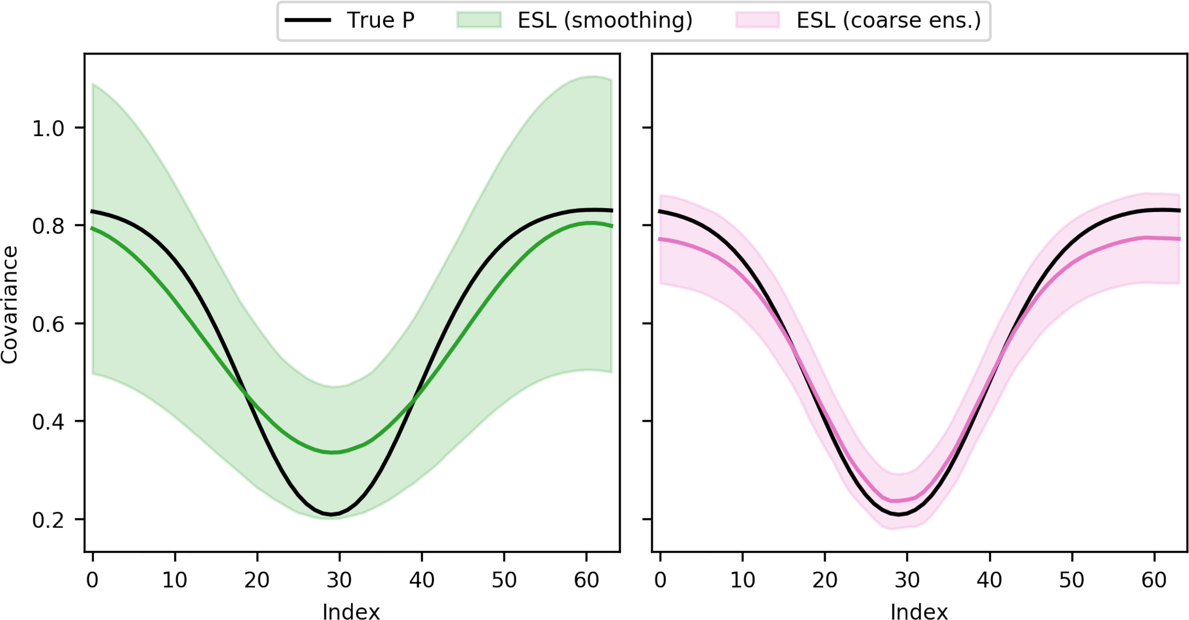
Fig. 6.
Comparison of ESL using smoothing (green, left) and a coarse ensemble (pink, right). Shown is the large-scale covariance of grid cells distanced five (fine-scale) grid points apart. The shaded areas represent the average plus and minus one standard deviation. Black: true covariance.
Table 1.
Errors in forecast covariance and analysis RMSE for ESL using smoothing or a coarse ensemble.
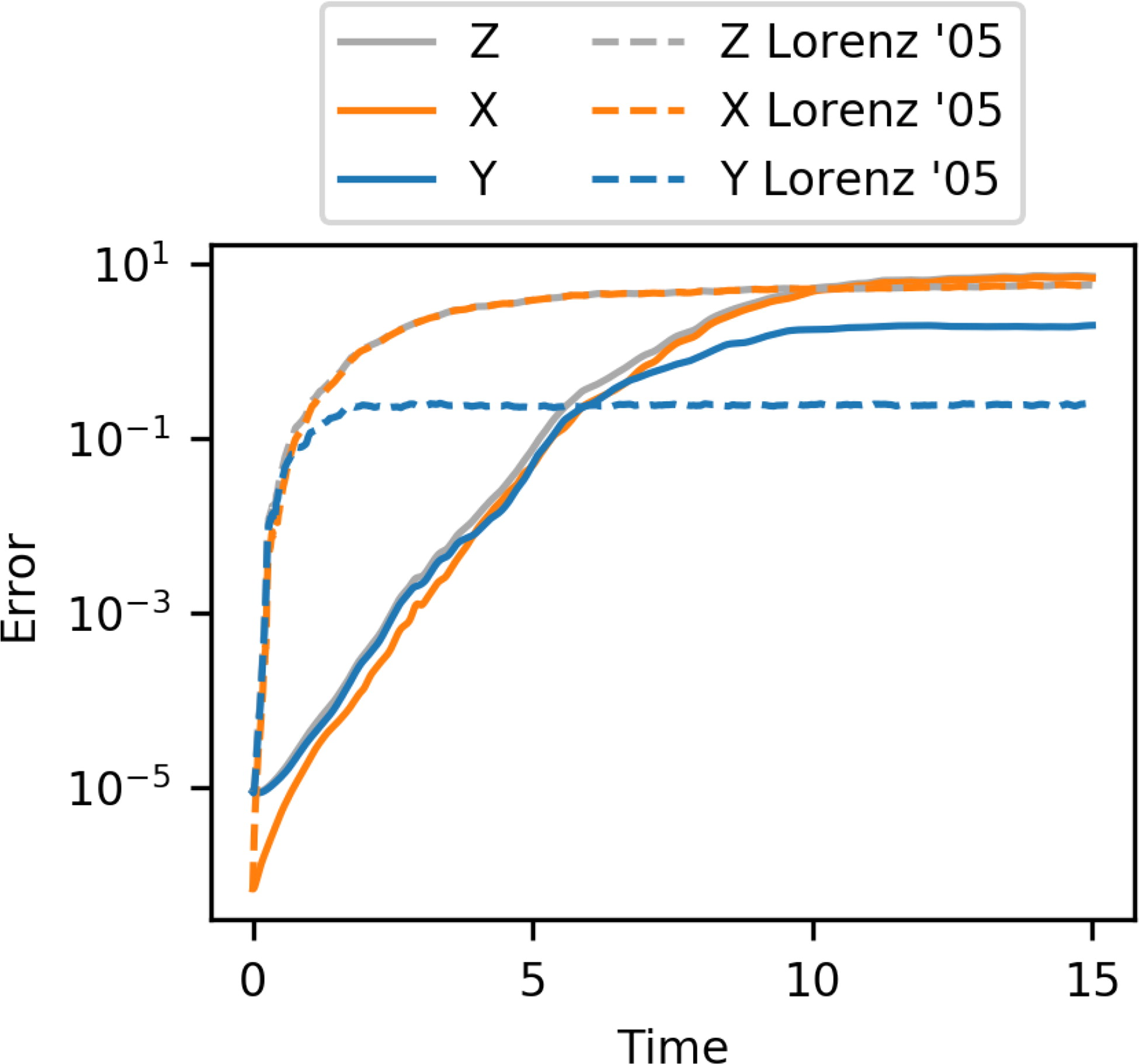
Fig. 7.
Error growth in Z (multiscale, grey), X (large scale, orange) and Y (small scale, blue). Solid lines correspond to LM3 with adjusted parameters. Dashed lines correspond to LM3 with parameters as in Lorenz (2005).
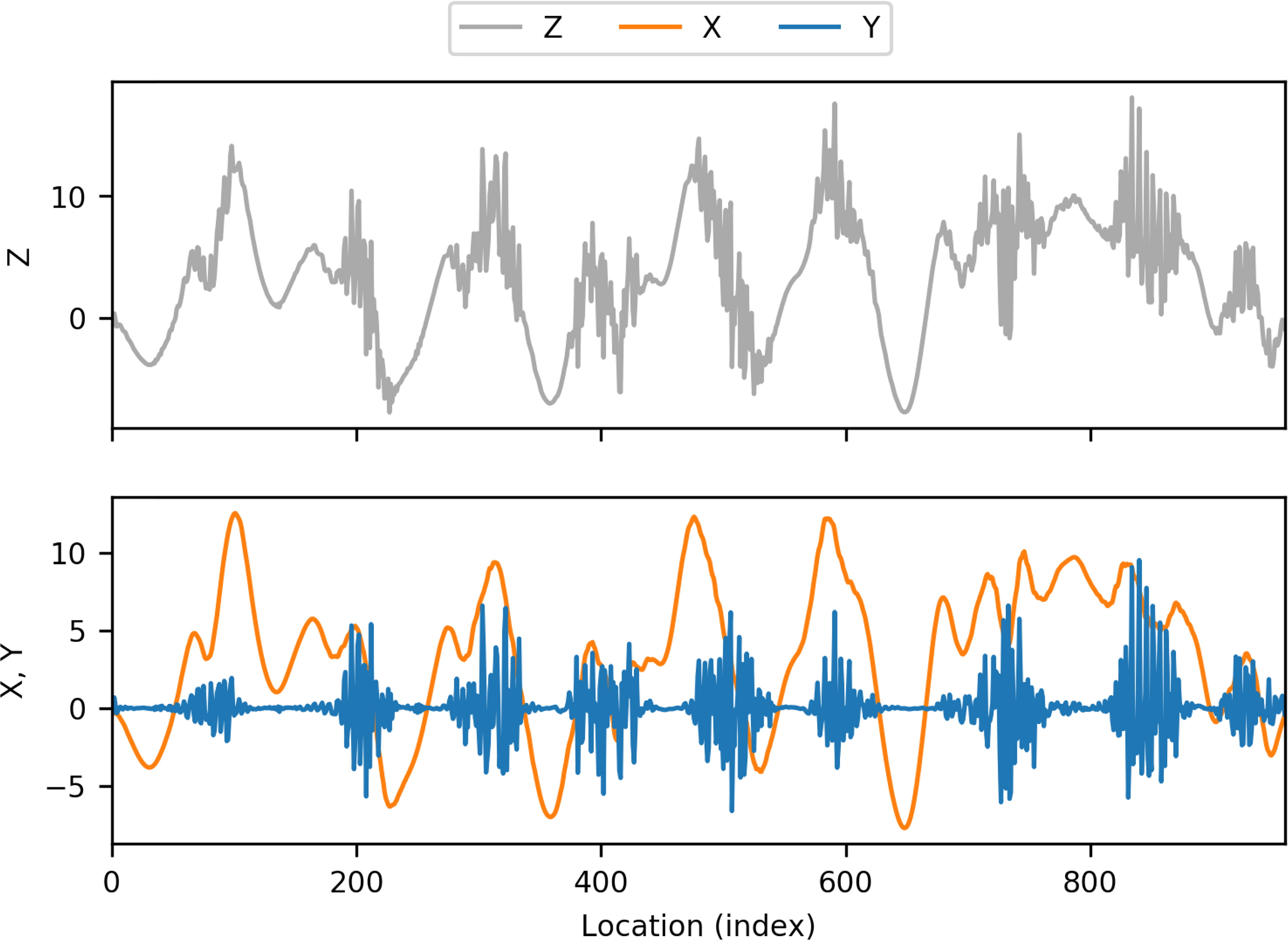
Fig. 8.
An example of a state of LM3 (adjusted parameters). Top (blue): multiscale variable Z. Bottom: large-scale variable X (orange) and small-scale variable Y (blue).
Table 2.
Parameters of the LM3 model.
Table 3.
Time averages of forecast RMSE and spread (tuned) for three localisation techniques.
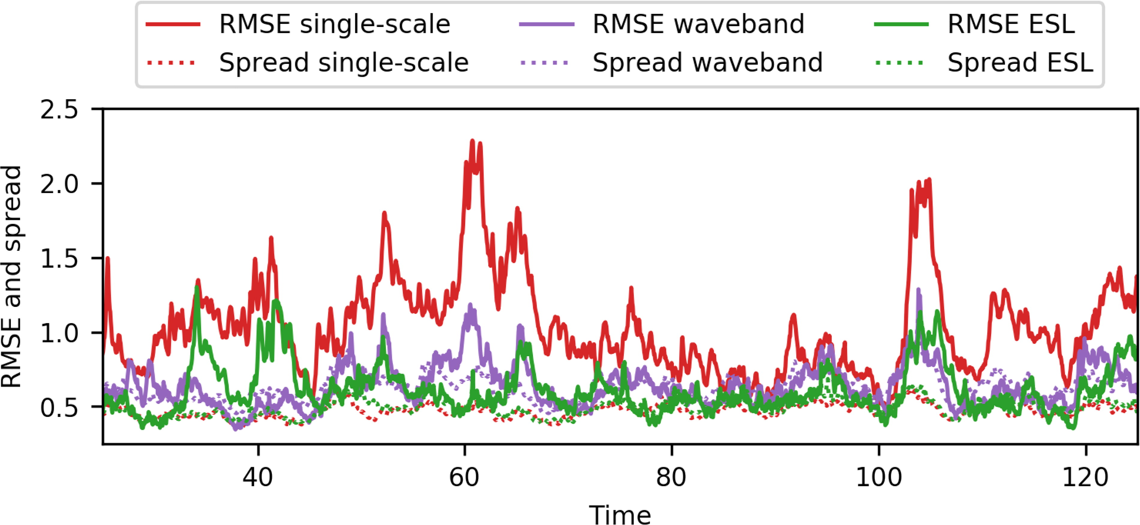
Fig. 9.
RMSE and spread in the multiscale variable Z of LM3 (after a 25 cycle spin up period). Solid lines: RMSE. Dashed lines: Spread. Red: single-scale localisation. Purple: waveband localisation. Green: ESL.