
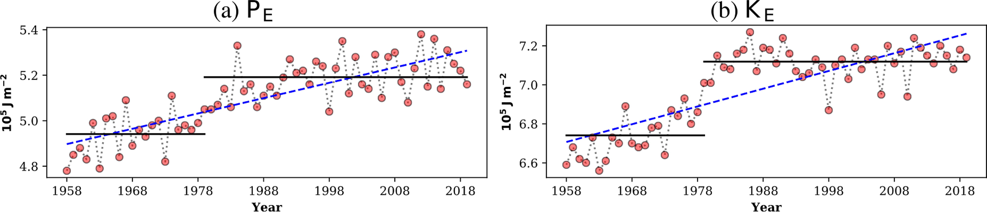
Fig. 1.
Variations of eddy available potential energy (PE ) and eddy kinetic energy (KE ) for JRA-55 data. Solid black lines are averages over 1958–1979 and 1979–2019, respectively. Unit is
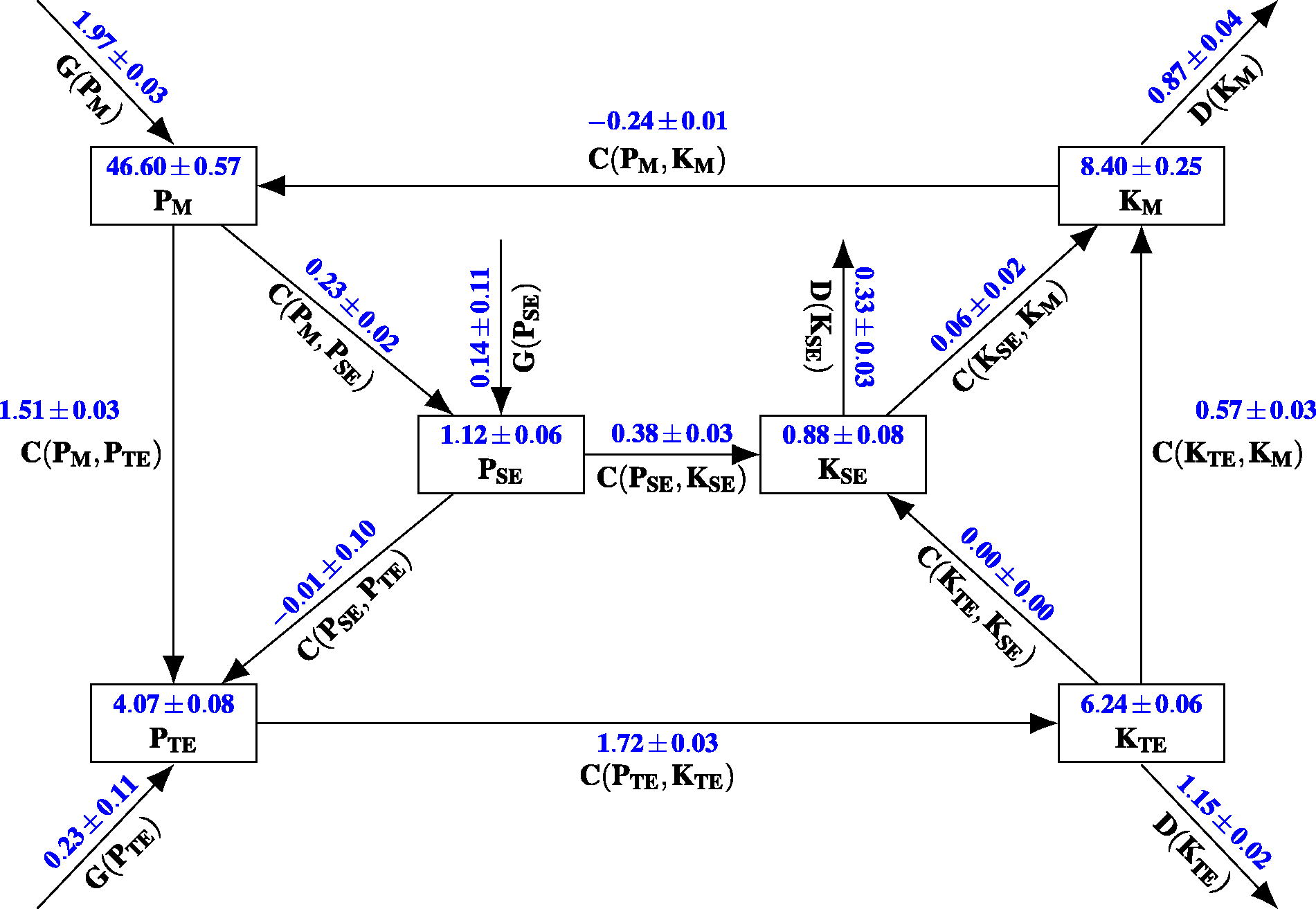
Fig. 2.
The Lorenz energy cycle diagram from JRA-55 reanalysis dataset during 1979–2019. The uncertain range of the time-mean values stand for the standard deviations of the time series of the energy components. Units are for energy and for the conversion rate, generation, and dissipation terms. The arrows indicate the direction that corresponds to positive values. Negative values imply the opposite direction.
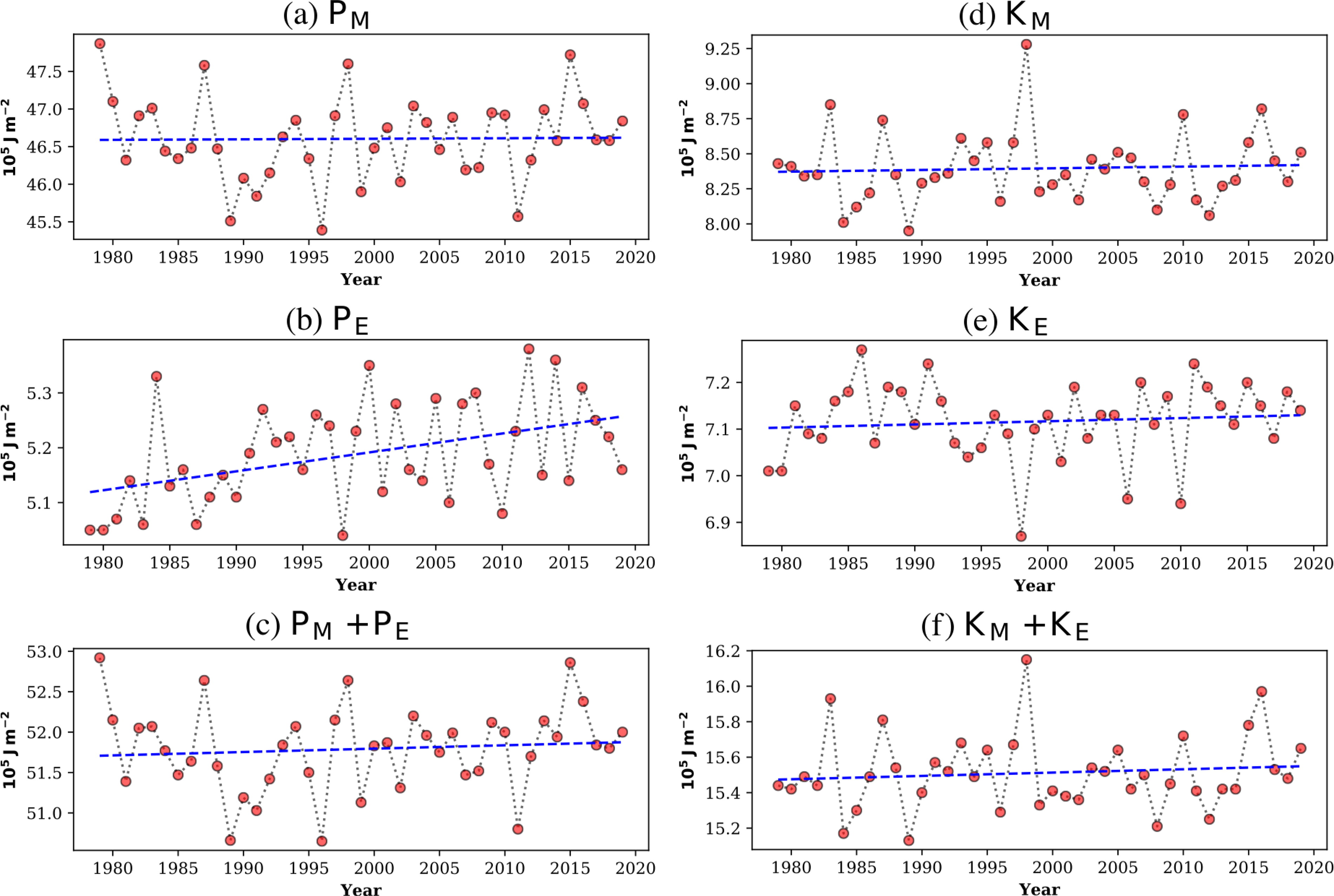
Fig. 3.
Time series of the globally averaged atmospheric energies. (a) The mean available potential energy PM . (b) The eddy available potential energy PE . (c) The total available potential energy (d) The mean kinetic energy K M. (e) The eddy kinetic energy KE . (f) The total kinetic energy
Table 1.
Trends in the global energies.
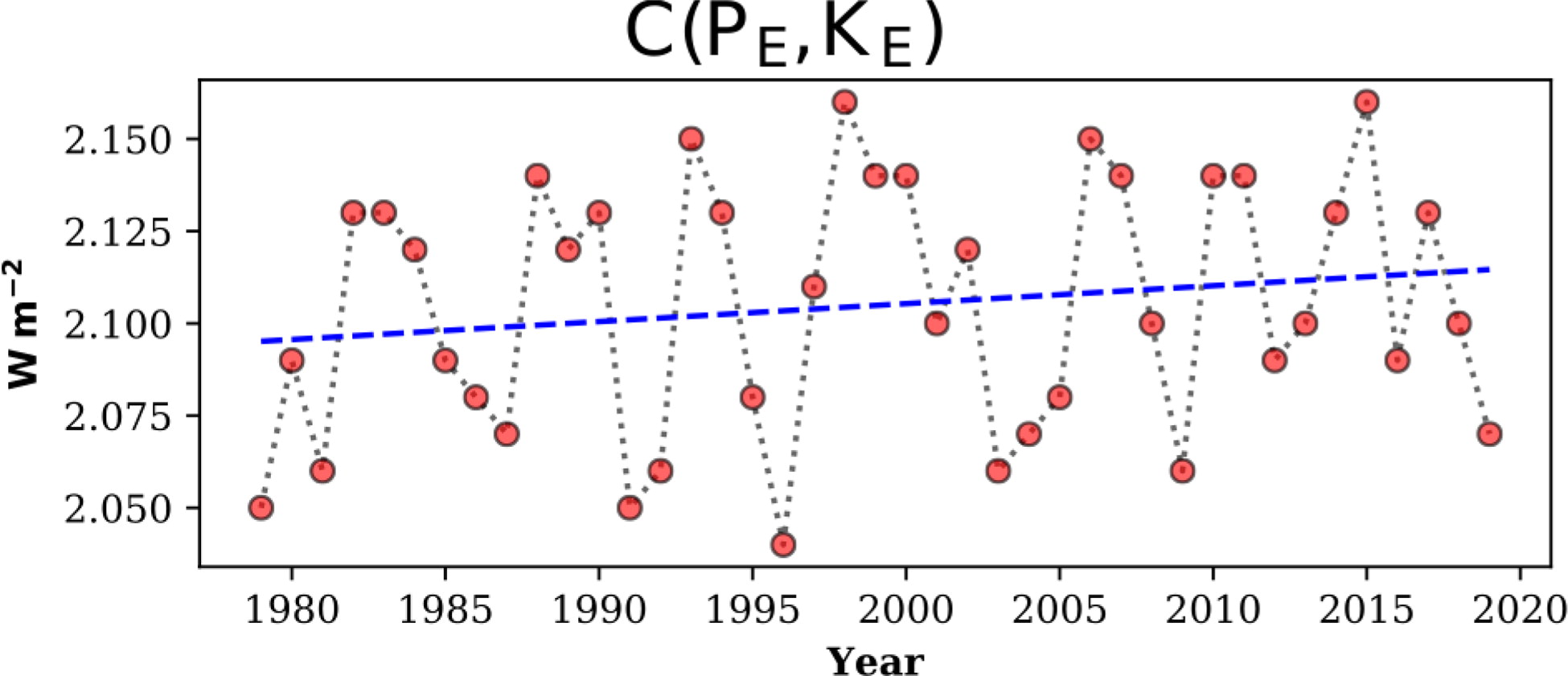
Fig. 4.
Time series of the conversion rate between the eddy available potential energy and the eddy kinetic energy
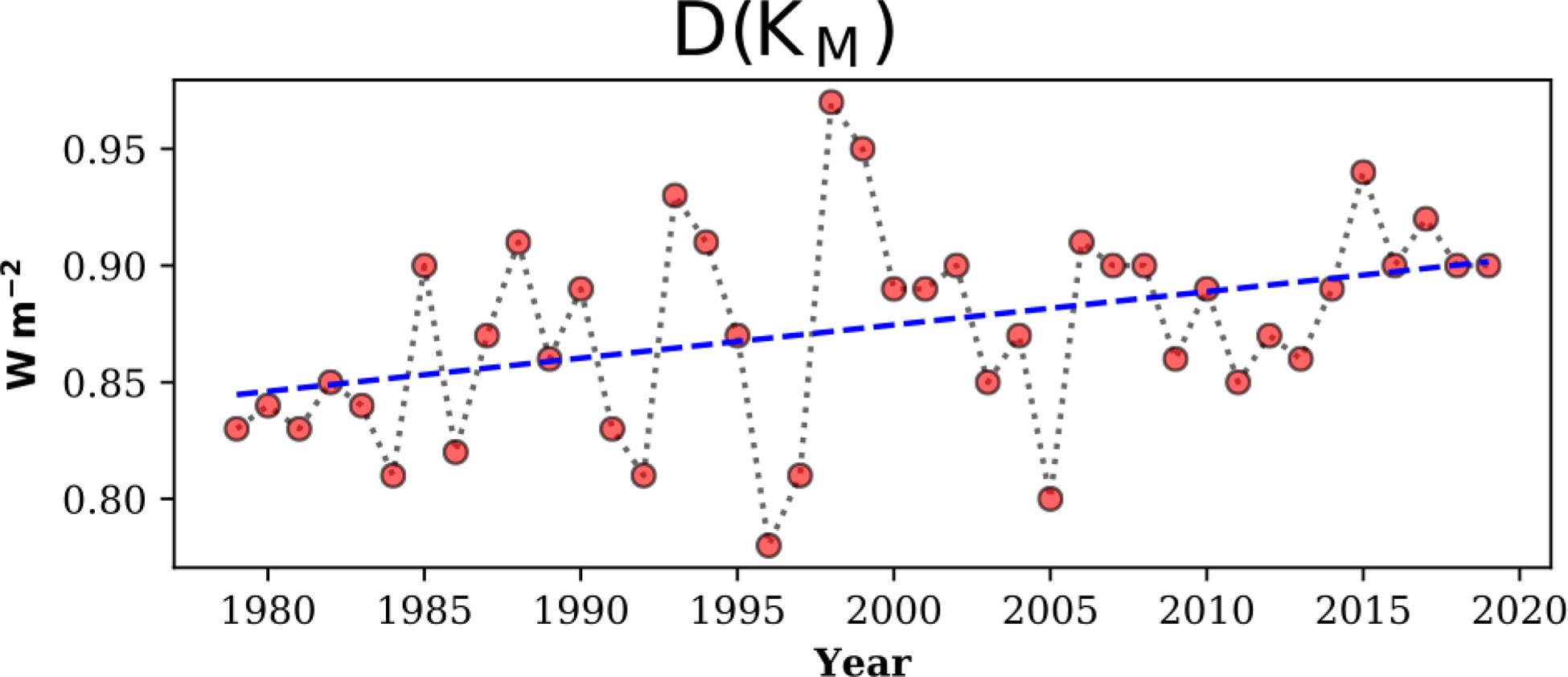
Fig. 5.
The dissipation rate of the mean kinetic energy
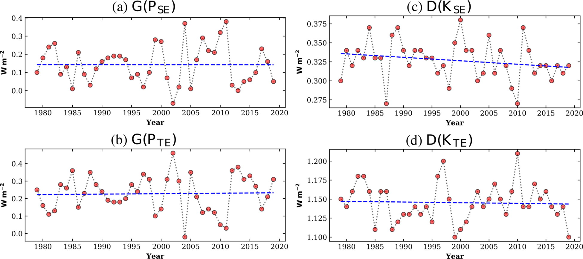
Fig. 6.
Decomposed globally averaged generation and dissipation rates. (a) The generation rate of the stationary eddy available potential energy (b) The generation rate of the transient eddy available potential energy (c) The dissipation rate of the stationary eddy kinetic energy (d) The dissipation rate of the transient eddy kinetic energy
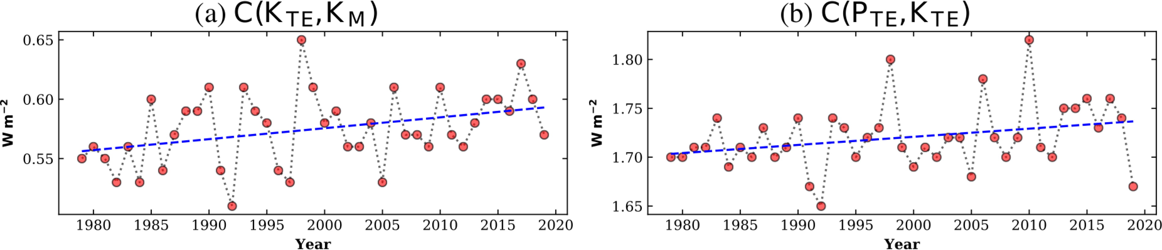
Fig. 7.
Decomposed globally averaged conversion rates. (a) The conversion rate between the transient eddy kinetic energy and mean kinetic energy (b) The conversion rate between the transient eddy kinetic energy and transient eddy kinetic energy
Table 2.
Decomposition of global energies into eddies.
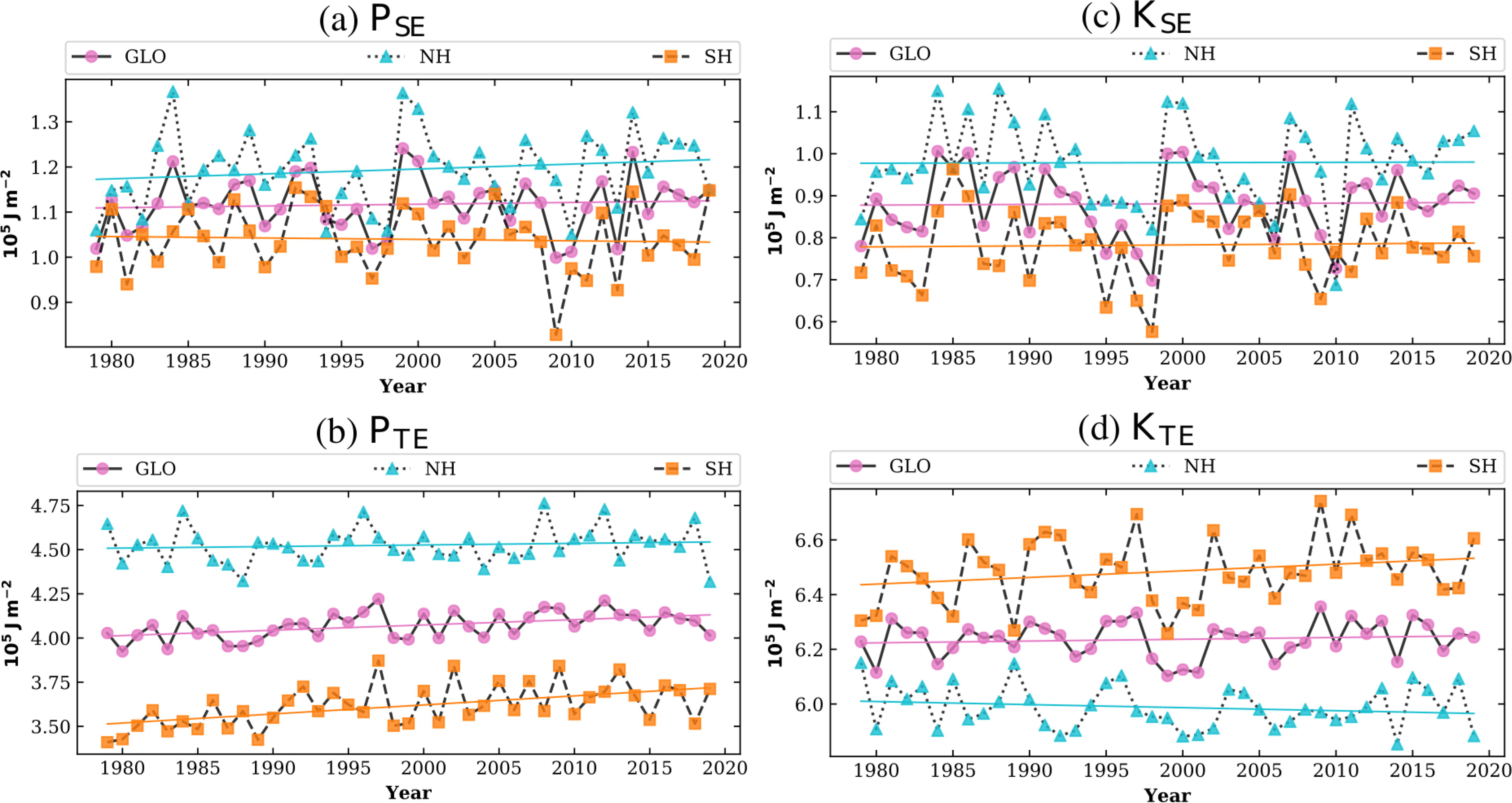
Fig. 8.
Decomposed the globally averaged eddy available potential energy and kinetic energy. (a) The stationary eddy available potential energy PSE ; (b) The transient eddy available potential energy PTE ; (c) The stationary eddy kinetic energy KTE ; (d) The transient eddy kinetic energy KTE .
Table 3.
Decomposition of potential and kinetic energy ( per year).
Table 4.
The climatological eddy available potential and kinetic energy on different wave-number domain during 1979–2019 ( per year).
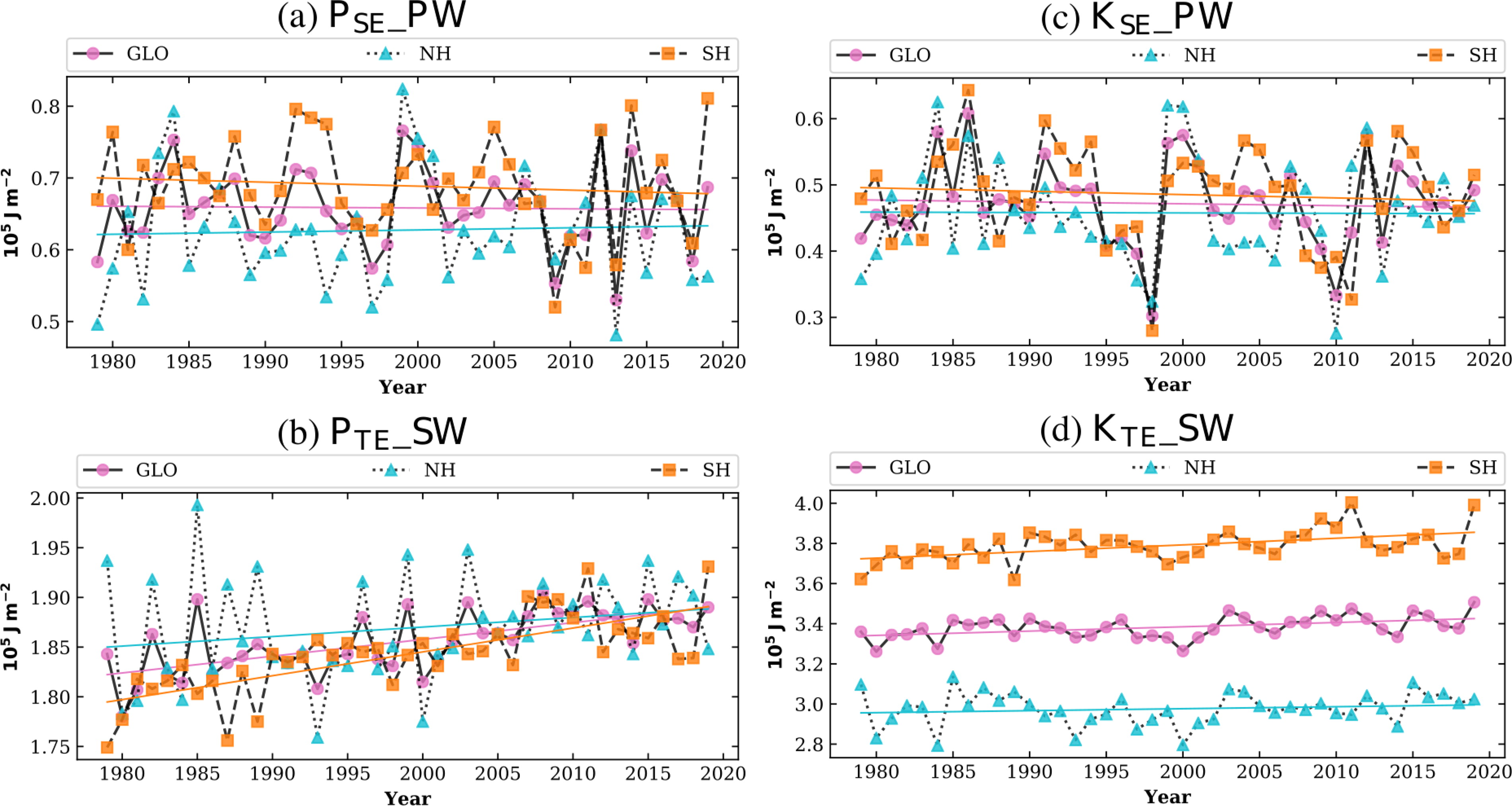
Fig. 9.
Decomposed the stationary and transient eddy energies into wave-number domain. (a) Energies in Planetary-scale Waves group for the stationary eddy available potential energy (b) Energies in Synoptic-scale Waves group for the transient eddy available potential energy (c) Energies in Planetary-scale Waves group for the stationary eddy kinetic energy (d) Energies in Synoptic-scale Waves group for the transient eddy kinetic energy
Table 5.
Decomposition of mechanical energy into wave number domain ( per year).
Table 6.
Correlations between climate indices and different global Lorenz energy cycle components.
Table 7.
Correlations between climate indices and different eddies Lorenz energy cycle components at different scales.