
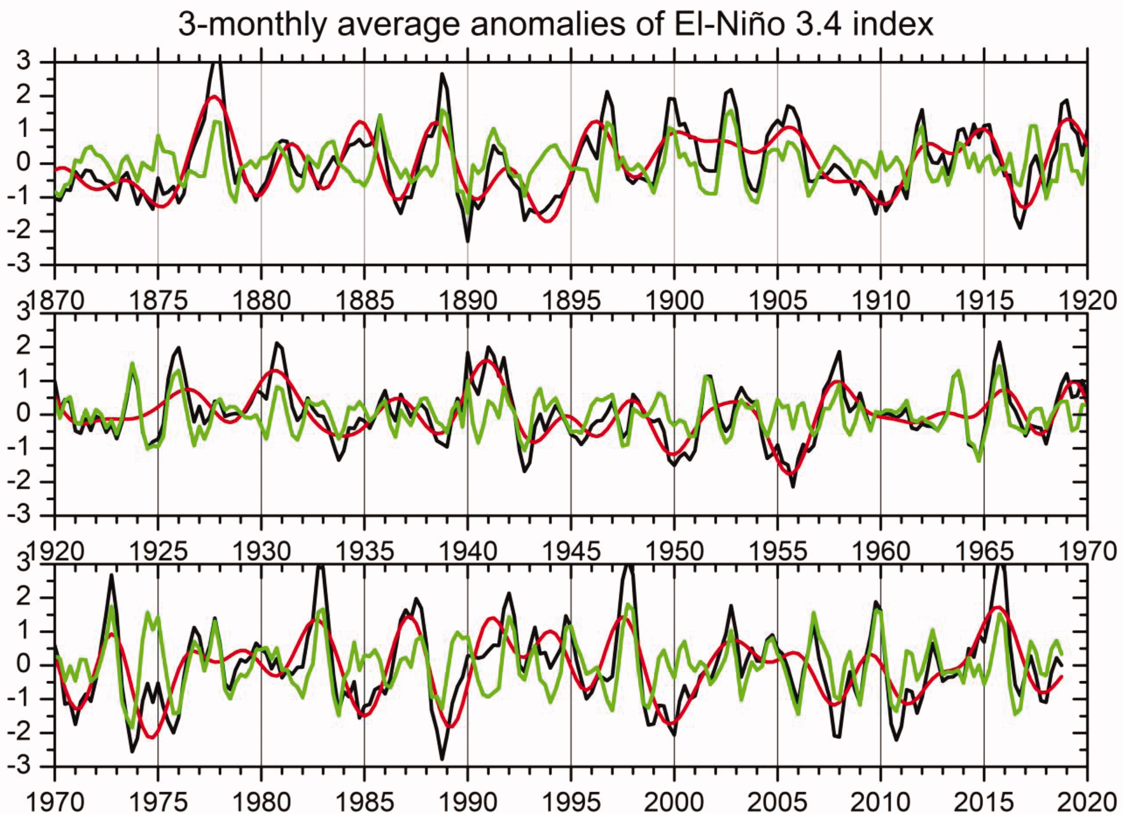
Fig. 1.
Detrended and standardized time series in the period 1870–2018, of the three-monthly average anomalies (with respect to the annual cycle) of El Niño 3.4 index (black) and its low-pass (red) and high-pass (green) components with a cutoff frequency of 0.08 cycles per trimester roughly corresponding, respectively, to inter- and intra-triennial timescales variability.
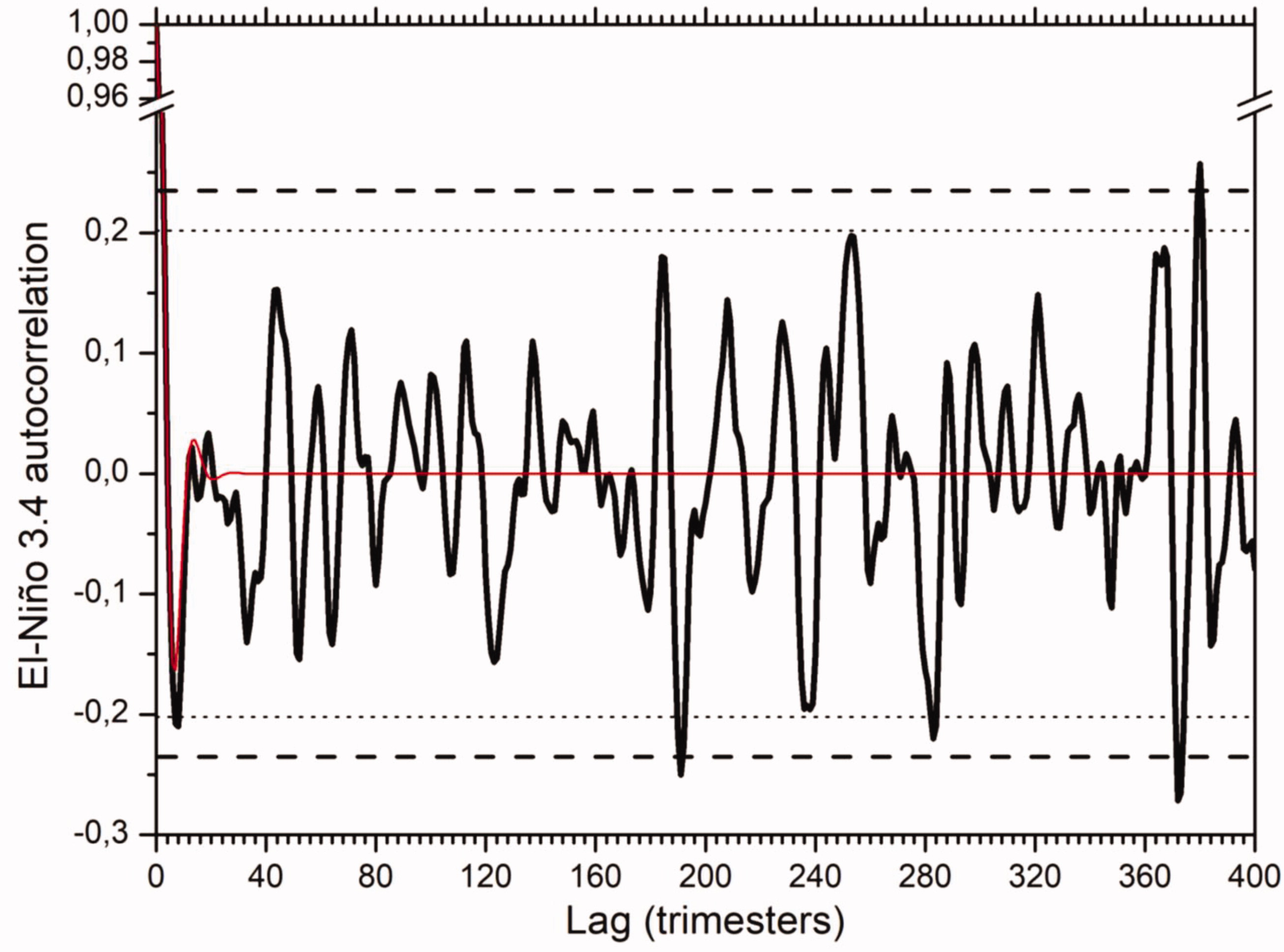
Fig. 2.
Autocorrelation function of El Niño 3.4 index (solid black) along with the 95% (dashed black) and 90% (dotted black) confidence interval. The autocorrelation function of the AR(5) model fitting data is also shown (solid red).
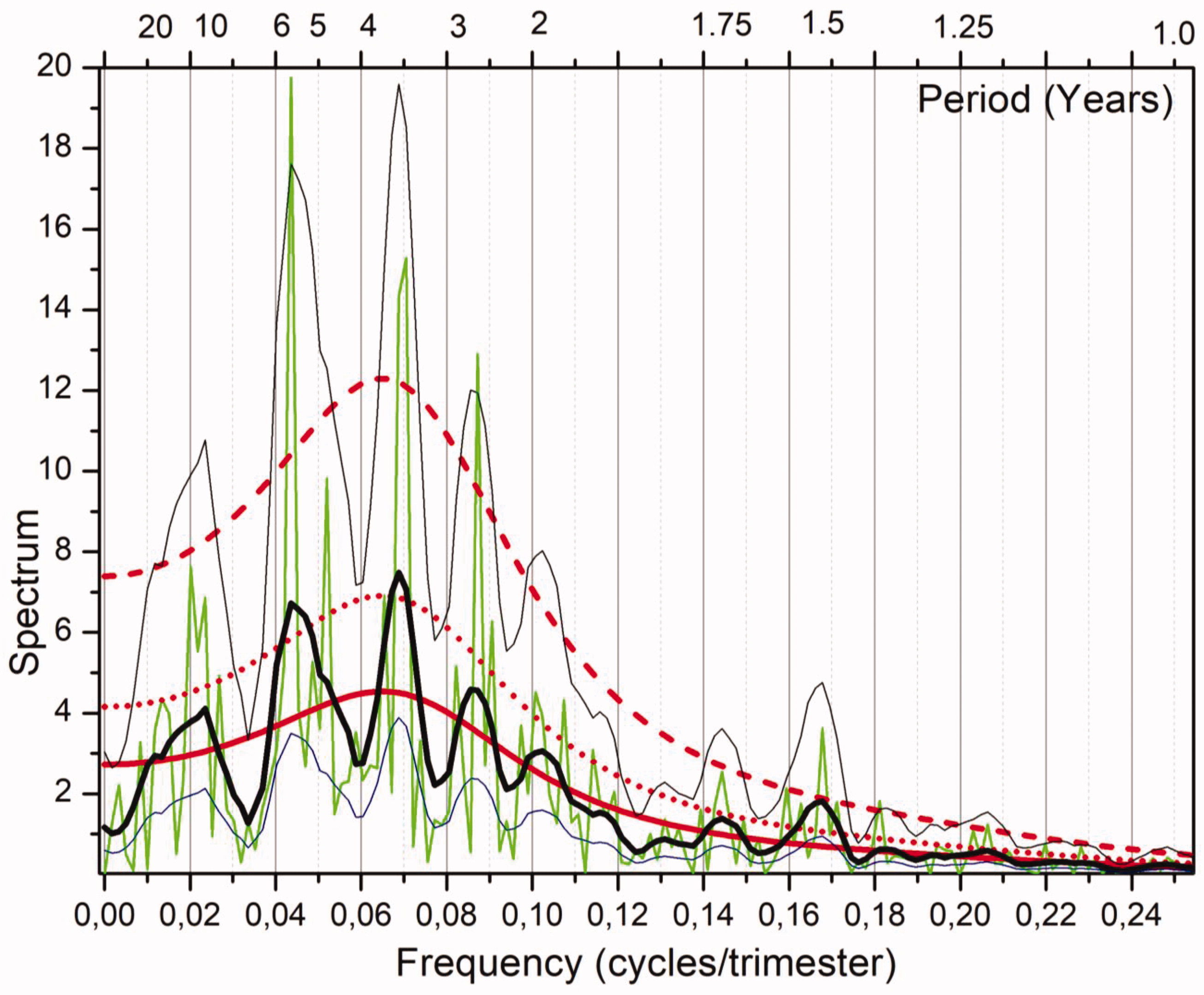
Fig. 3.
Empirical periodogram (thin green); Smoothed spectrum (thick black) and corresponding 95% confidence interval (thin black); theoretical AR(5) spectrum (red), and 10% significance level for the periodogram (red dashed) and for the smoothed spectrum (red dotted). Units are (°C)2/cpt. The top axis presents periods in years.
Table 1.
Values of the Akaike Information Criterium where is the residual noise variance of an AR(p) model fitting.
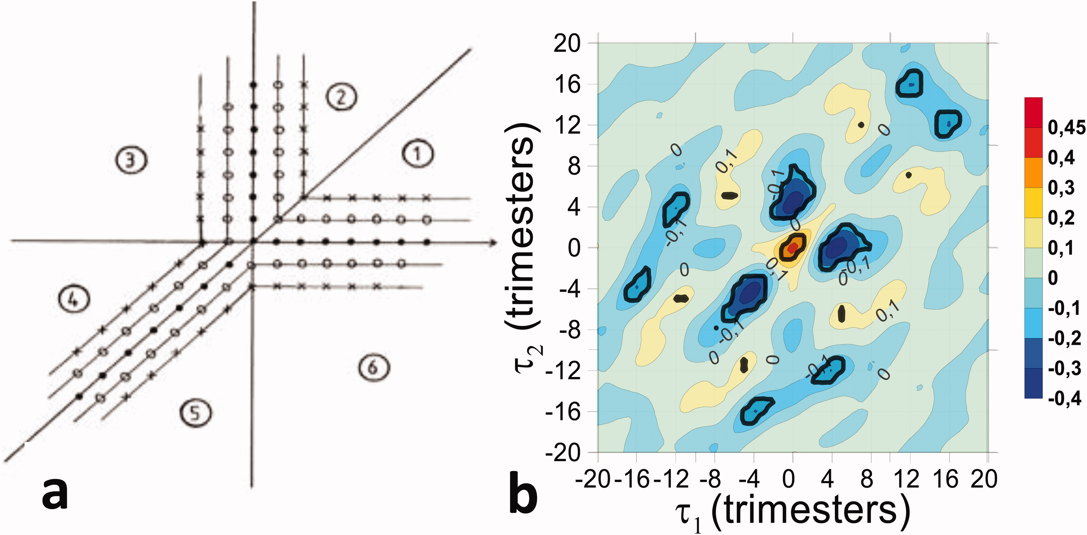
Fig. 4.
Symmetries (a) of the bicovariance function in the delay plan (adapted from Rao and Gabr, 1984) and bicorrelation of El Niño 3.4 index (b). Thick black contours show the 5% significance level.
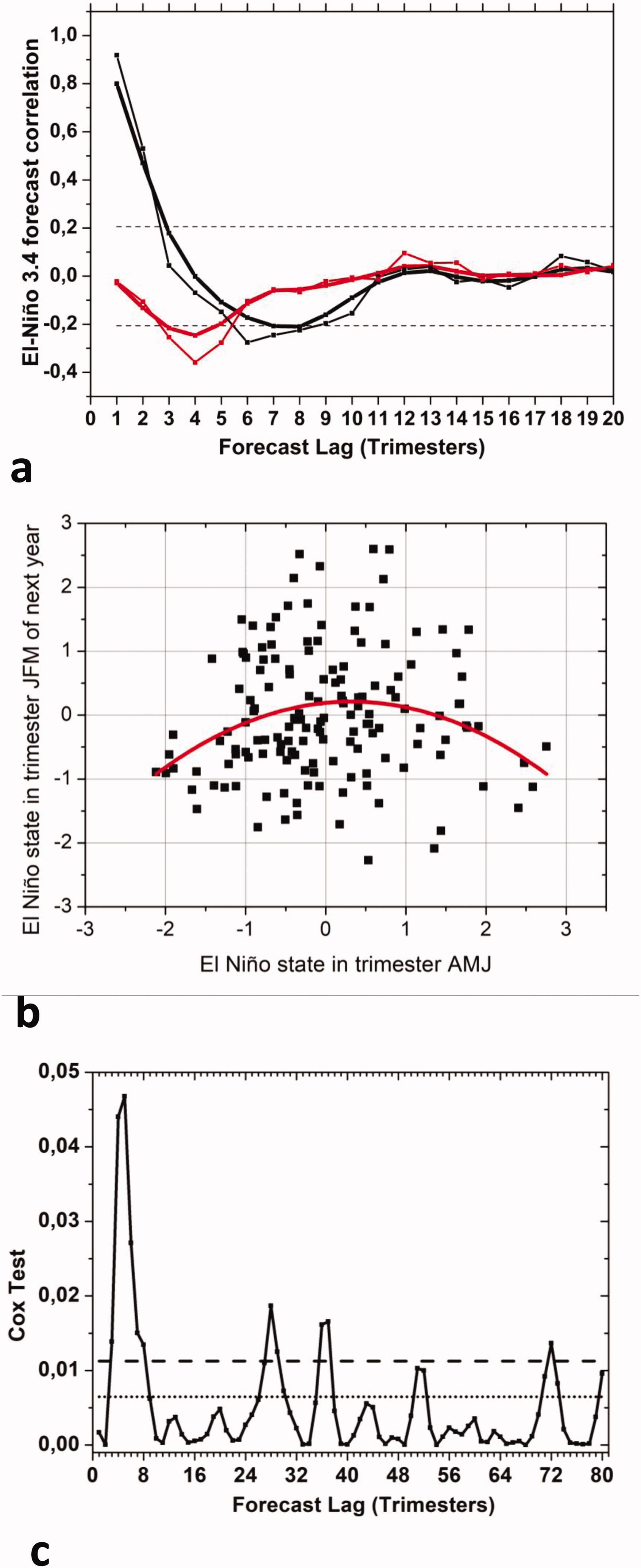
Fig. 5.
(a) Linear (thick black) and nonlinear (thick red) correlations ( and respectively) of El Niño 3.4 index. The same correlations restricted to forecast trimester JFM (black thin and red thin respectively). Horizontal dashed lines show the 10% significance level interval (b) AMJ versus following year JFM El Niño and best quadratic fitting. (c) Cox test (thick) and the 95% (dotted) and 99% (dashed) confidence level threshold of nonrejection of the linearity hypothesis.
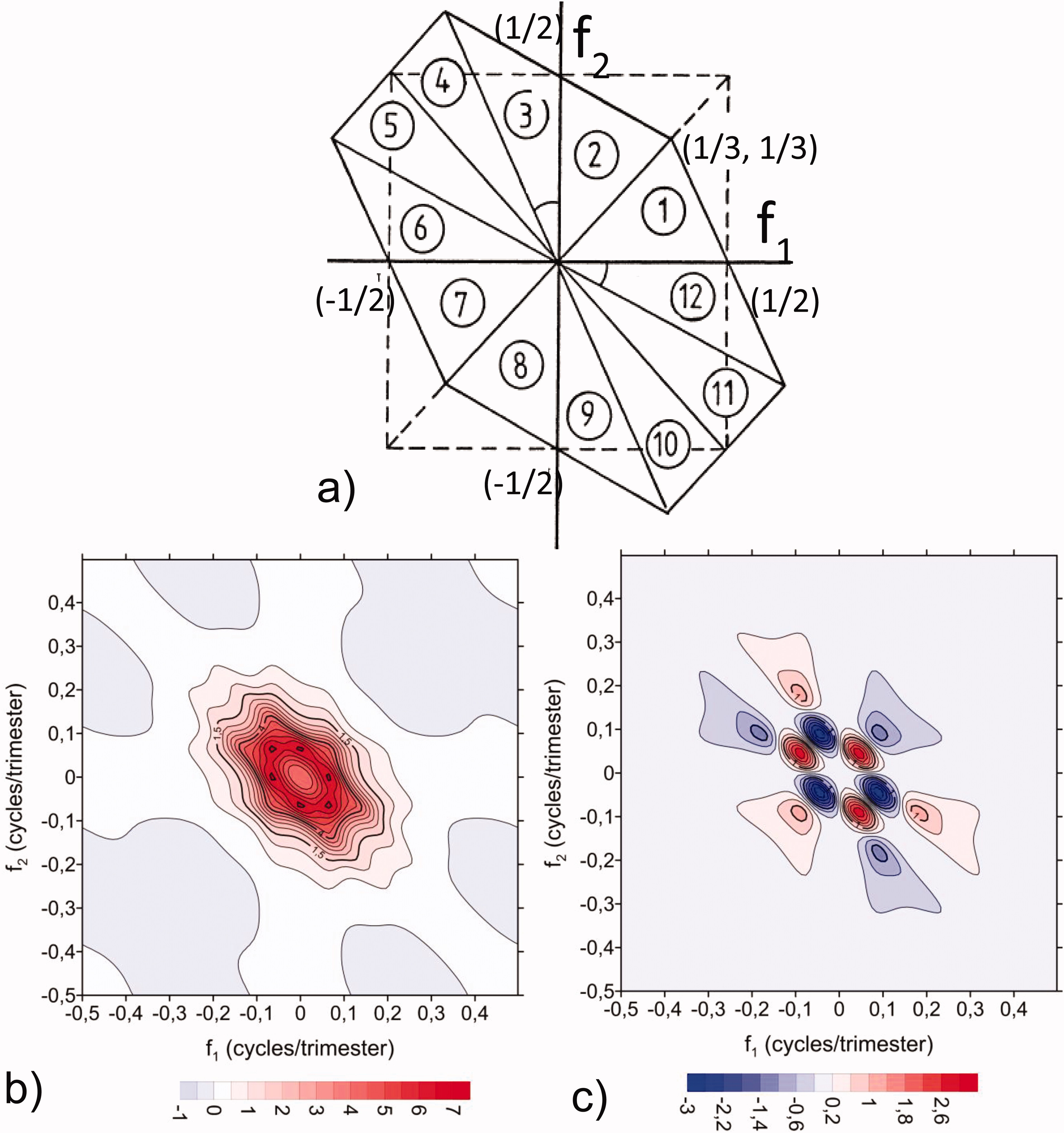
Fig. 6.
Principal domain (triangle 1) in the spectral plane and its symmetric replicas (a) (adapted from Rao and Gabr (1984). Real (b) and Imaginary (c) parts of the bispectrum of the NGAR(5) model. Note the symmetries associated with the 12 sectors shown in panel a).
Table 2.
Average fluctuations of the bispectrum and the average confidence interval half-size (CIHS) for several values of the window length (Eq. (A4)).
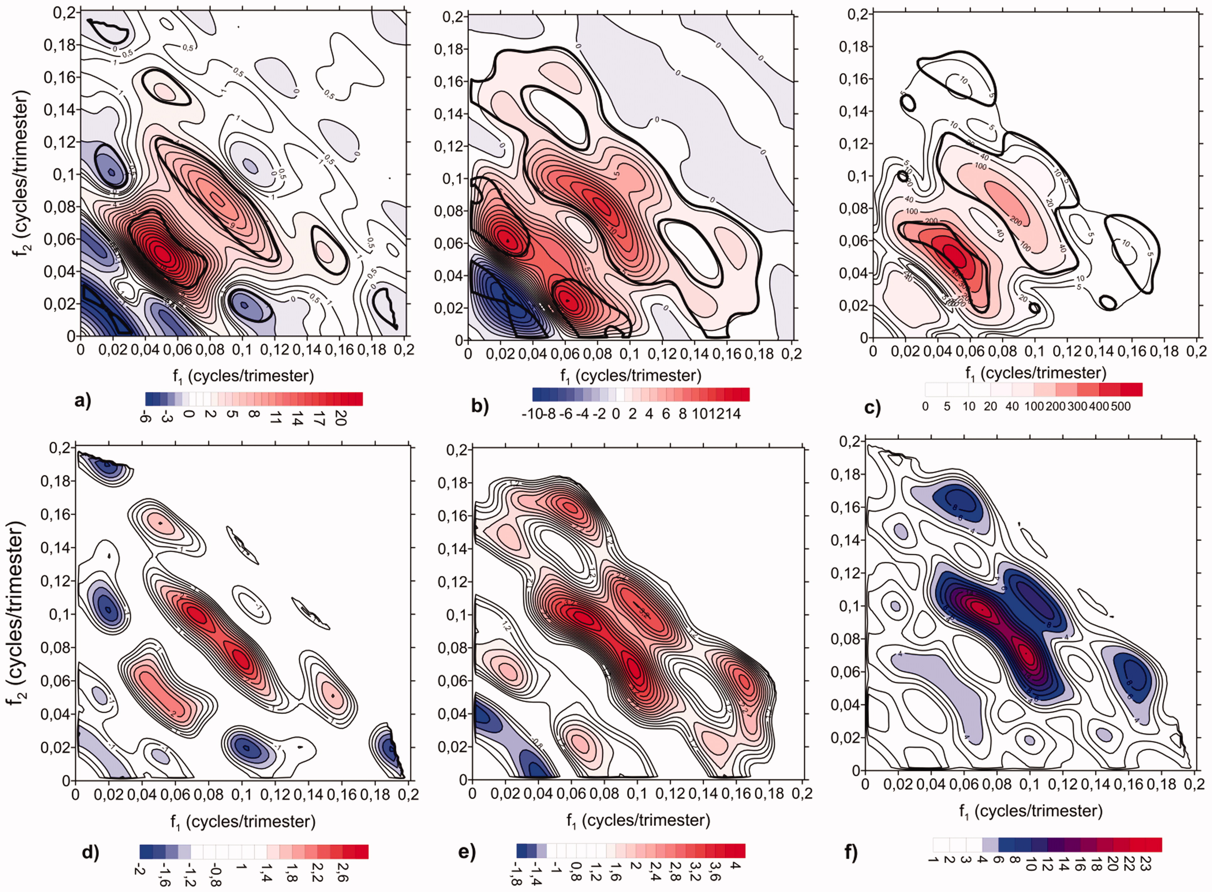
Fig. 7.
Real (a) and Imaginary (b) part of the empirical bispectrum using a window lag (M 2 =30). Squared amplitude of the smoothed bispectrum (c). In figures a–c, significant regions at 20% significance level (or lower) appear within thick contours. Real (d) and imaginary (e) parts of the standardized bispectrum deviation of El Niño index, and corresponding sum of the squared real and imaginary parts (f). Bifrequencies for which the null hypothesis is rejected at 20% significance levels (or lower) are color-shaded ( for each part). Values are restricted to the most significant part of bispectrum.
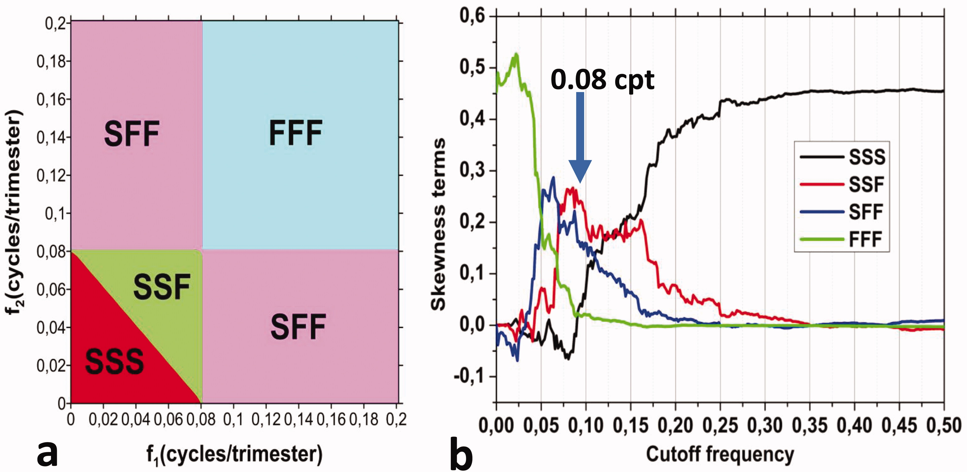
Fig. 8.
(a) Subdomains SSS, SSF, SFF and FFF obtained from a frequency partition using a cut-off frequency cpt (∼3 years). (b) Contributing terms to El Niño 3.4 index skewness (Eq. (26)).
Table 3.
Contributing terms to skewness, Eq. (26), obtained from time series and from partial integrals of the smoothed bispectrum: total, negative and positive contributions. The most relevant integral positive (negative) contributions are marked in bold, representing the most relevant types of interaction contributing to extreme El Niño (La Niña) events.
Table 4.
Expected values (yellow) of the third moment of the normalized El Niño 3.4 index (denoted as sk) and its contributions SSS, SSF, SFF and FFF, as detailed in Eq. (26) for the full period and for the three half centuries 1870–1919 (HC1), 1920–1969 (HC2) and 1970–2018 (HC3). The expectations and their bispectral contributions are further decomposed into contributions conditioned to La Niñas (blue) and conditioned to El Niños (red). Note that (idem for skewness terms).
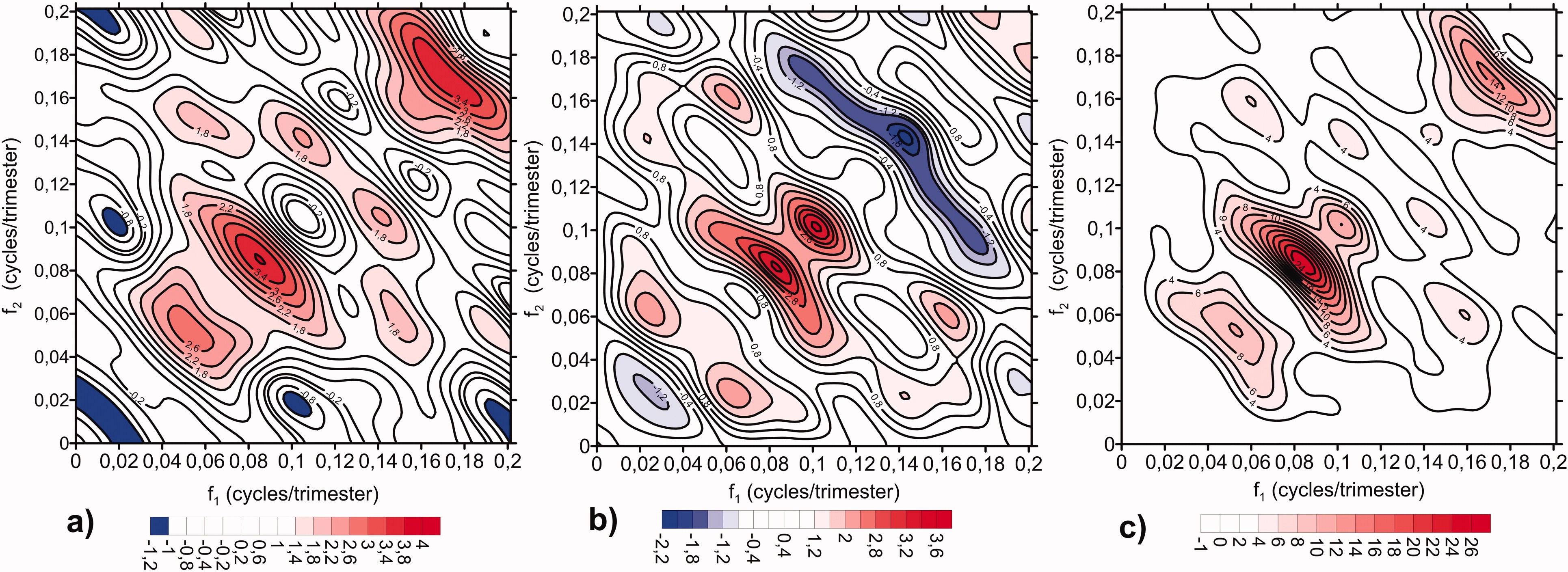
Fig. 9.
Real (a) and Imaginary (b) parts of the normalized smoothed bispectrum of El Niño index, (M 2=30) and its squared amplitude (c). Regions statistically significant at 20% level are colour-shaded.
Table 5.
Statistics of the AR(5) and bilinear ARBL(5,1),…,ARBL(5,5) models with the corresponding bilinear-term lags along with the terms and for simple and hybrid fitting in addition to the normalized AIC relative to hybrid fitting. Correlation skills are also shown at lags trimesters, assessed over the period 1970–2018 for models obtained by hybrid fitting calibrated in the period 1870–1969.
Table 6.
Coefficients and lags of the autoregressive and bilinear terms of the ARBL(5,5) model of El Niño index, obtained by hybrid fitting over the full period. The independent constant and the additive driving noise is
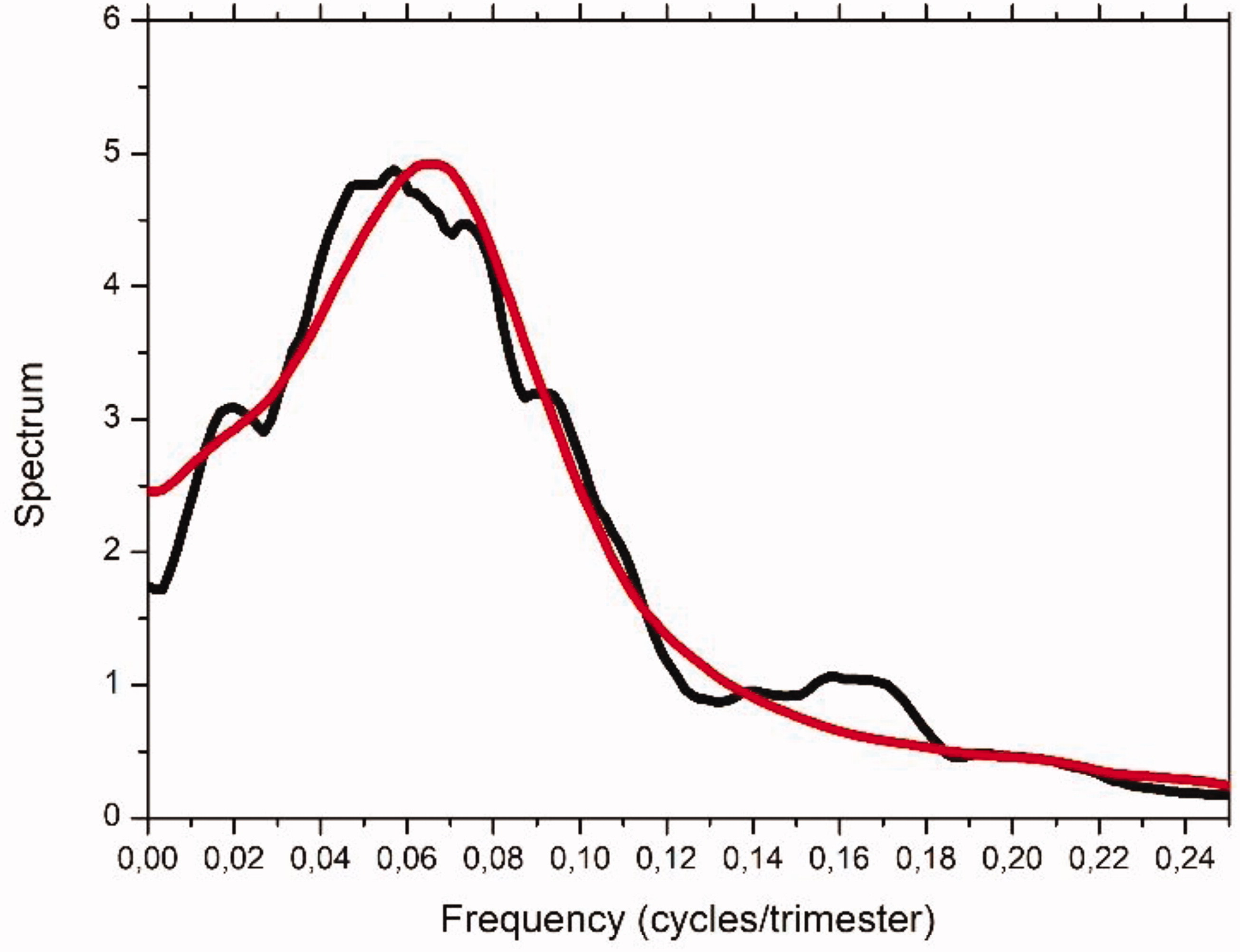
Fig. 10.
Smoothed empirical (black) and ARBL(5,5) simulated (red) spectra using a window lag M = 30.
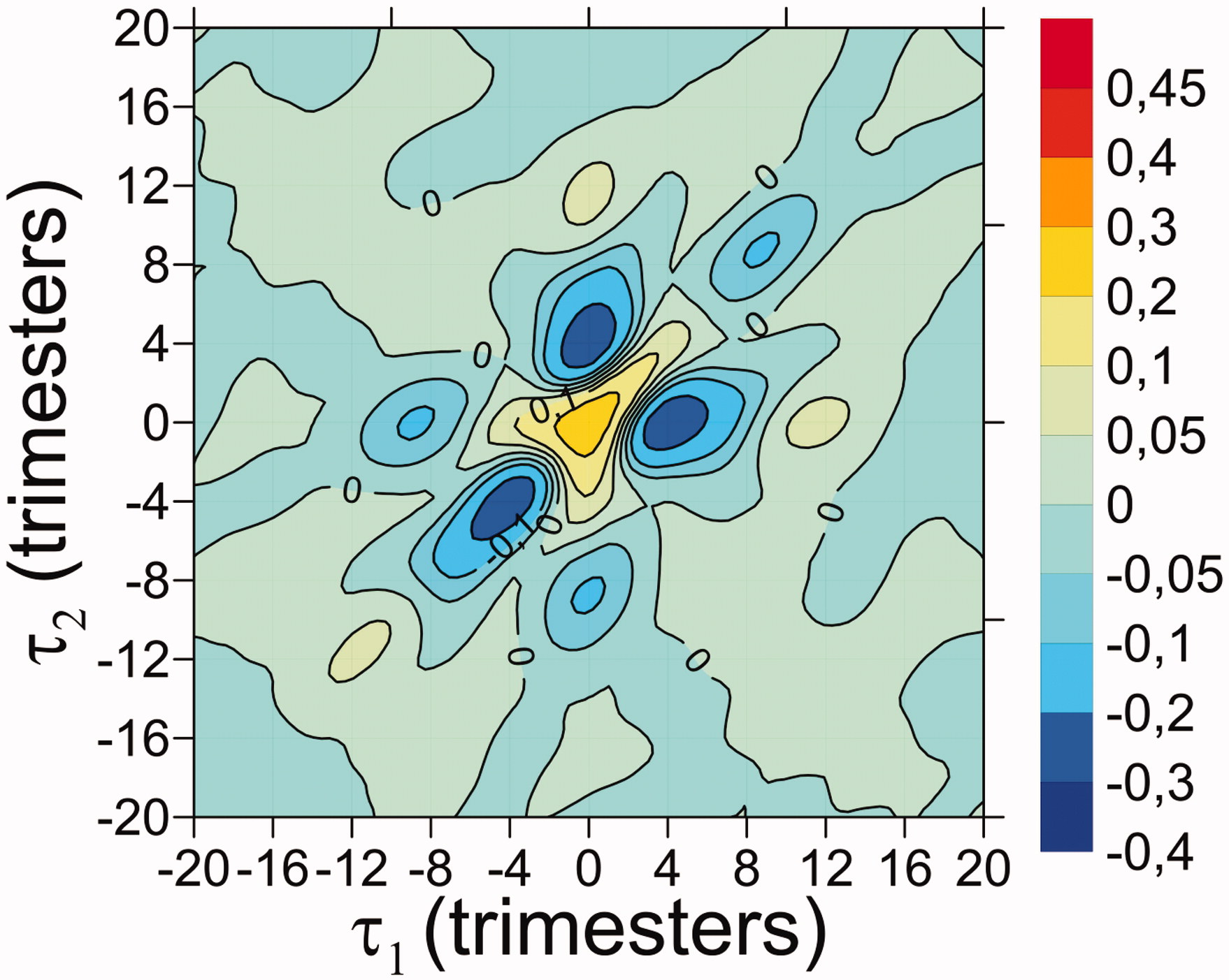
Fig. 11.
Bicorrelation of the ARBL(5,5) model, approaching the empirical bicorrelation of El Niño index (to be compared with Fig. 4b).
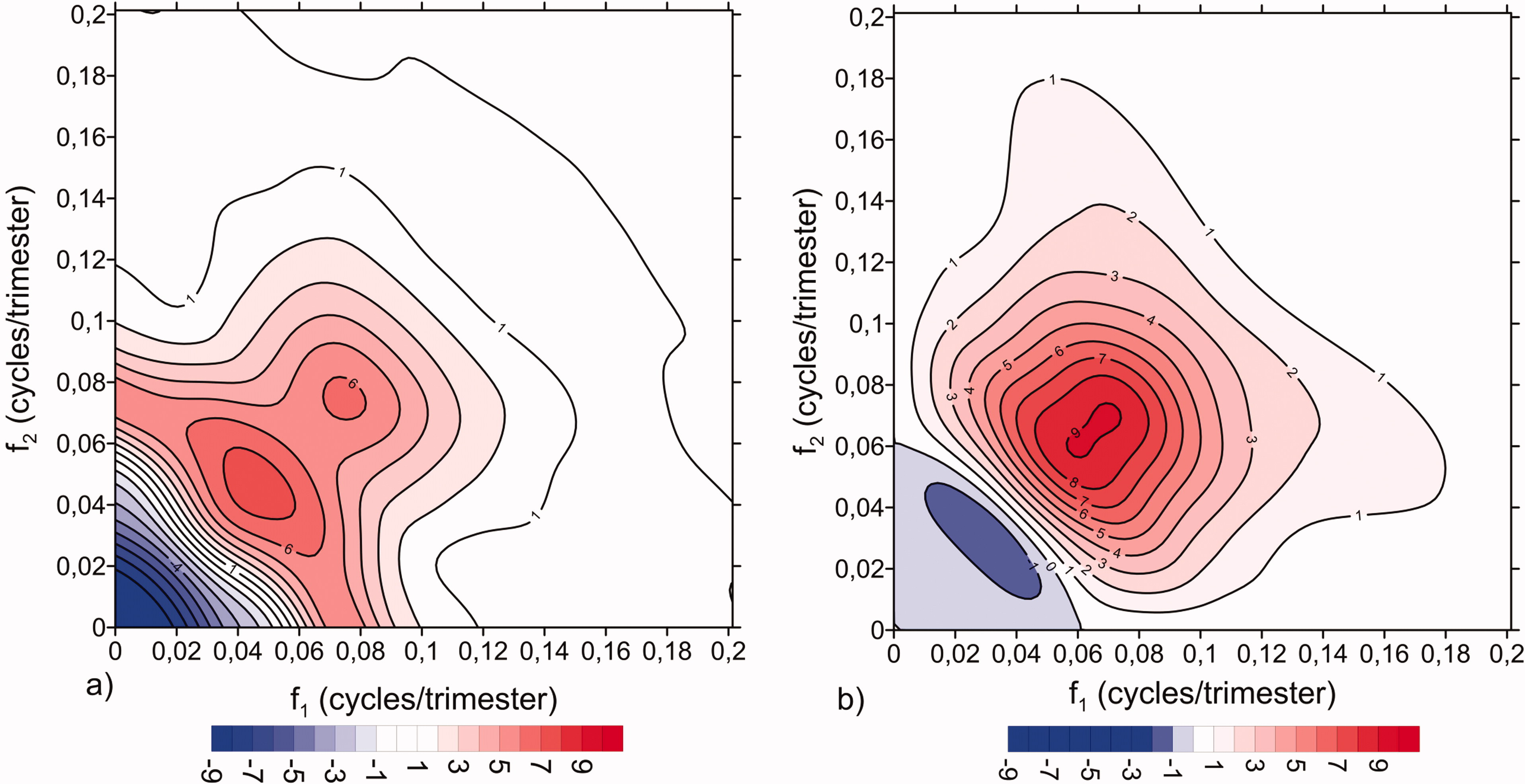
Fig. 12.
Real (a) and Imaginary (b) parts of smoothed bispectrum of the ARBL(5,5) using a window lag M 2=30.
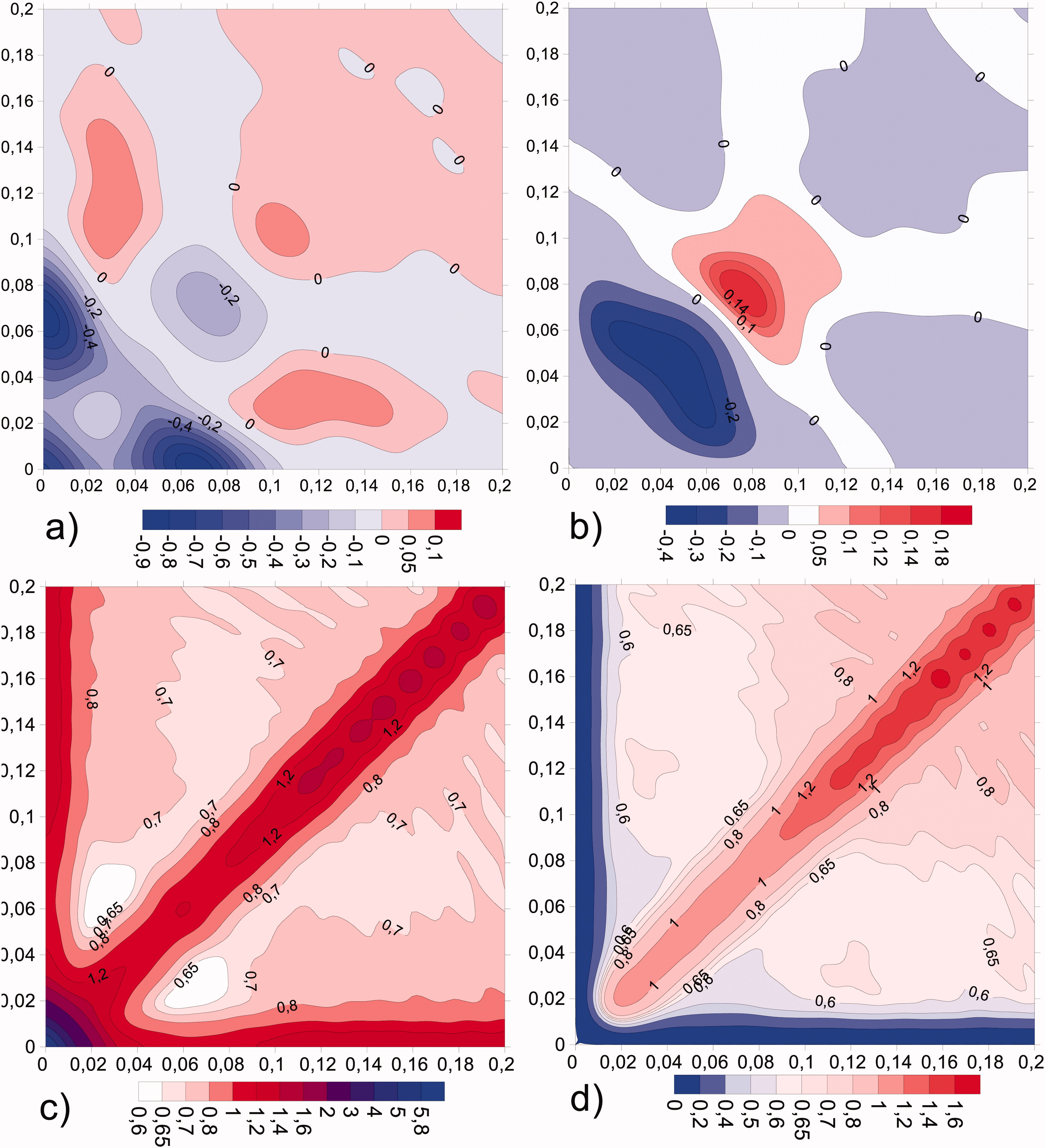
Fig. A1.
Real (a) and imaginary (b) parts of bias Real (c) and imaginary (d) values of the ratio between empirical variances and total asymptotic variance.
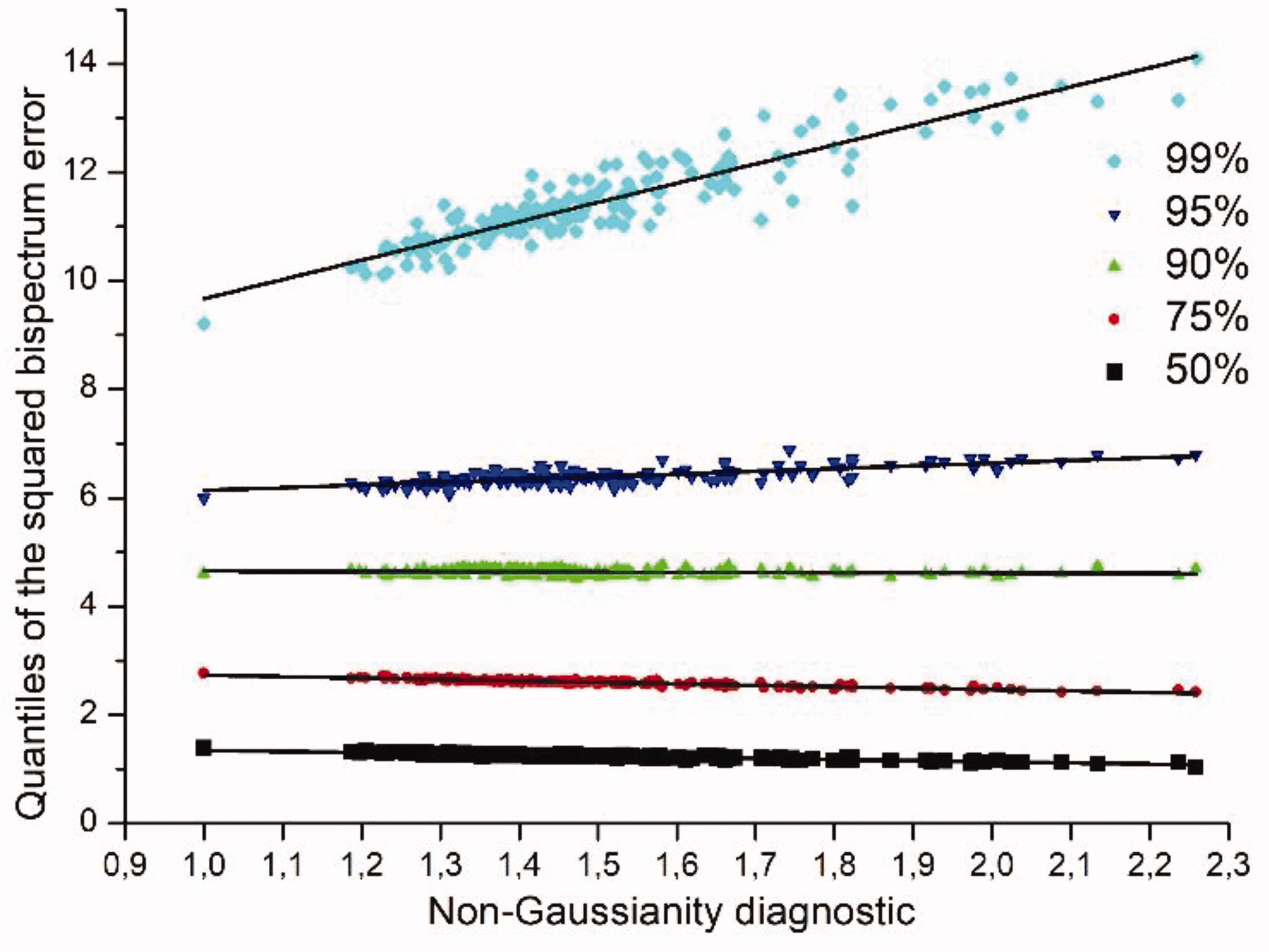
Fig. A2.
Values of the non-Gaussianity diagnostic (equal to 1 under Gaussianity) versus the 50%, 75%, 90%, 95% and 99% half-quantiles of the squared bispectrum normalized error, collected over all the 173 bifrequencies of lattice A linear adjustment is shown for each quantile.
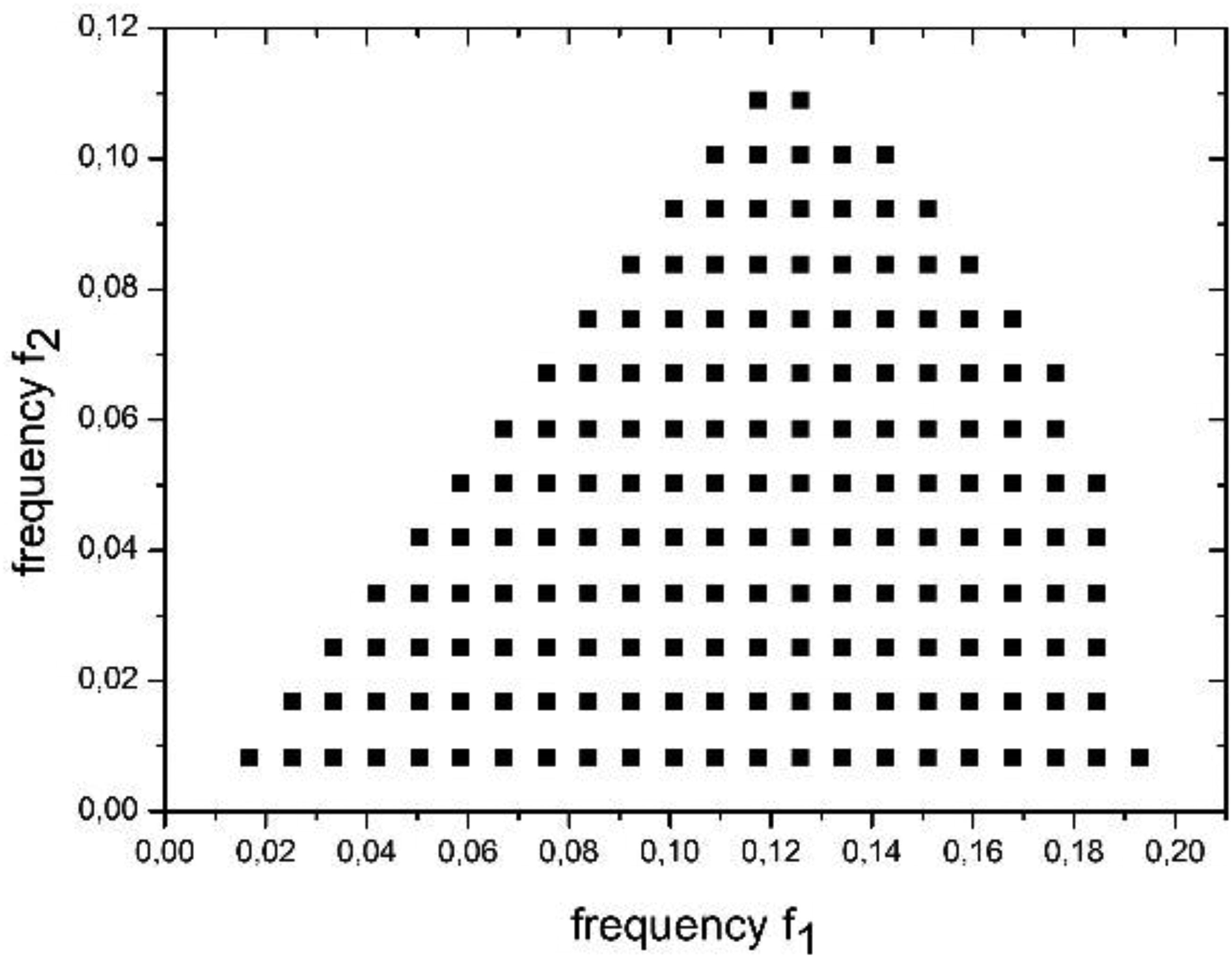
Fig. A3.
Position of bifrequencies in the set used in the integral test of linearity.