
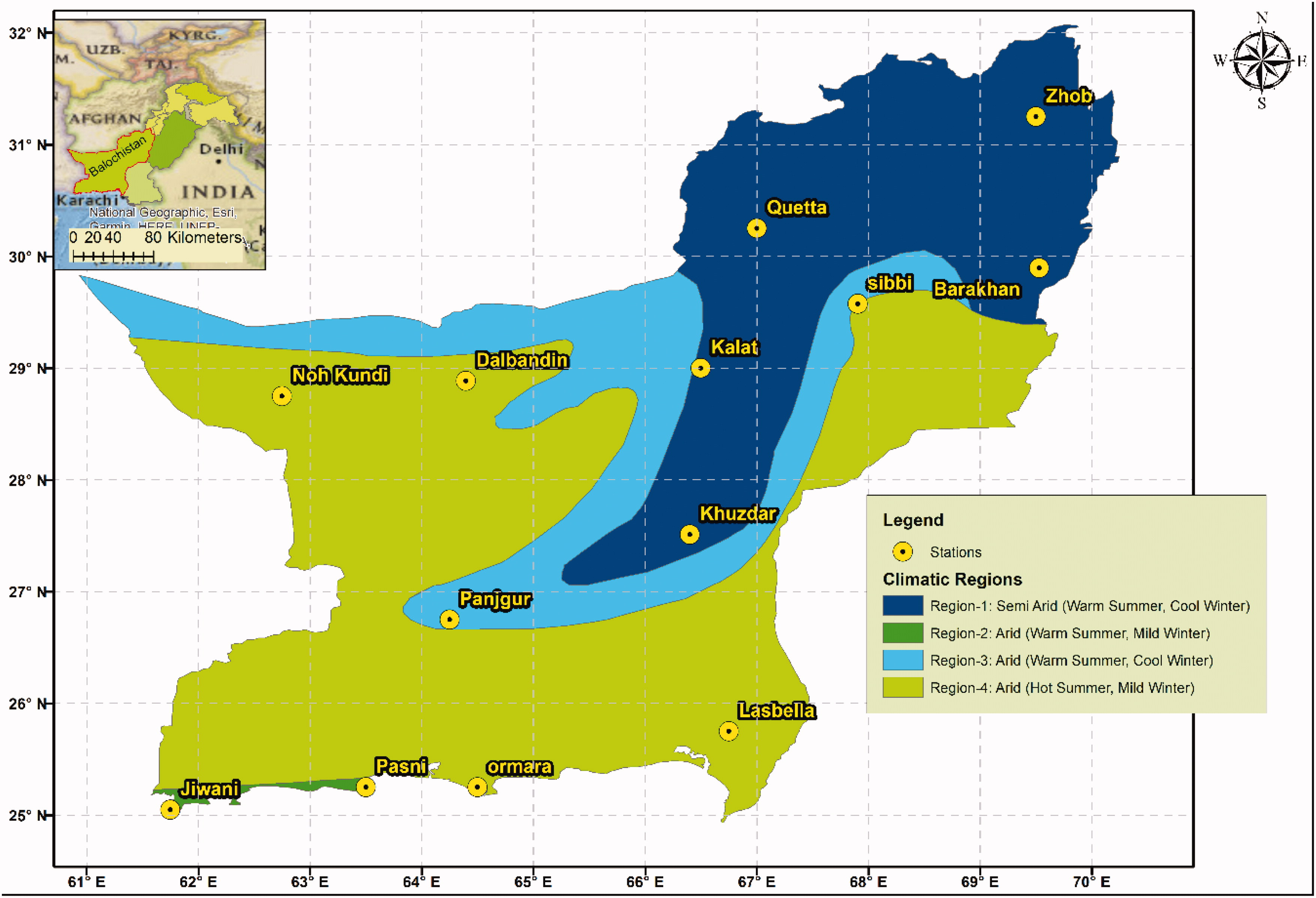
Fig. 1.
Study area and location of selected PMD stations in Baluchistan with regional distribution (Pakistan Climate Map, 2013).
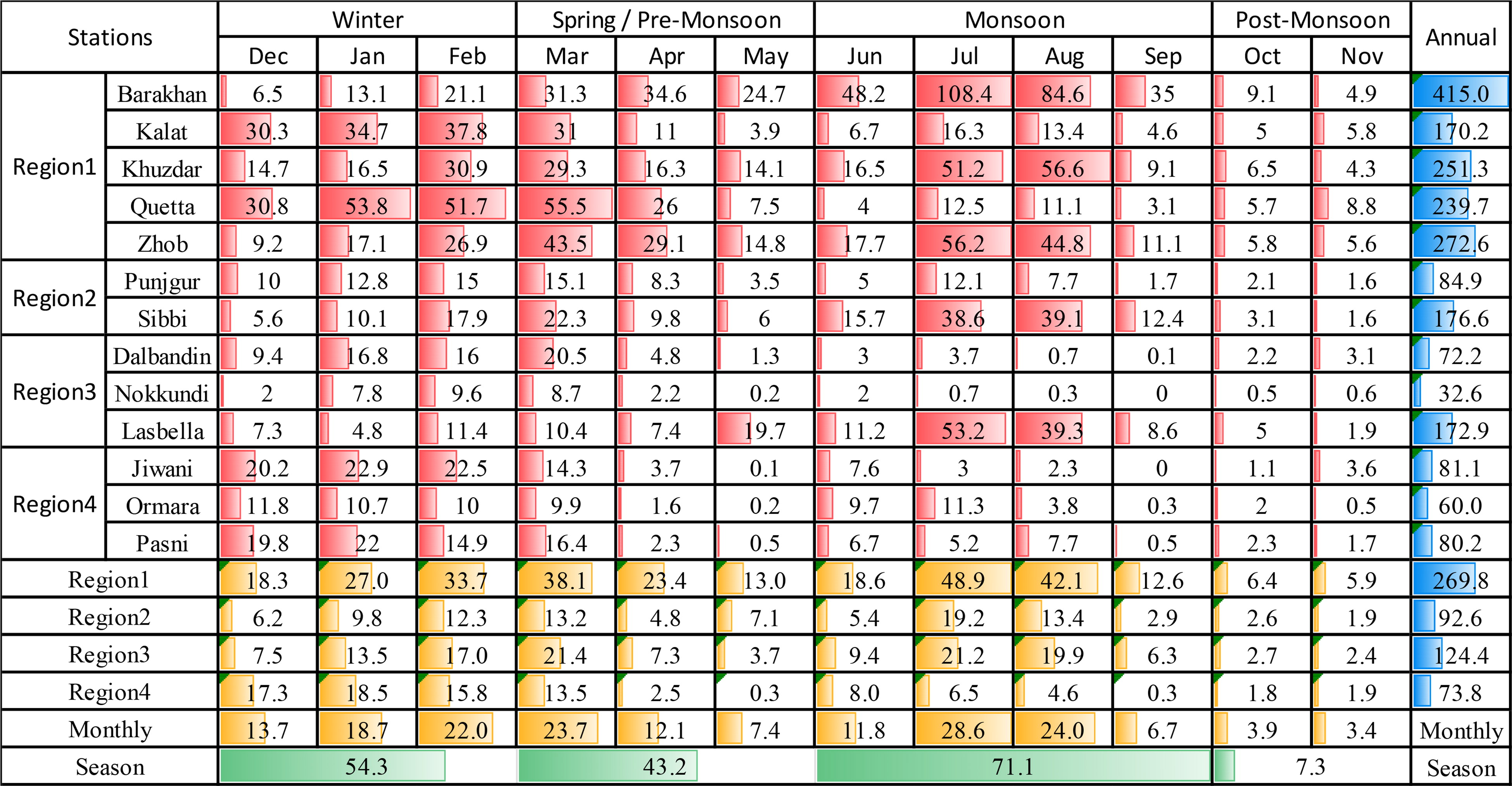
Table 2.
Description of climate indices.
Azores High: 25N-315, 30N-315, 45N-355, 50N-355; approx.AOwww.esrl.noaa.govArtic Poles; North of 20NAMOwww.esrl.noaa.gov0-60N; 280–360 approx.DMIwww.jamstec.go.jp/aplinfo/sintexf/e/index.htmlEEIO; 0-10S; 90–110
WEIO; 10N-10S; 50–70EQWINwww.esrl.noaa.govCEIO: 5N-5S; 60–90ENSO-MEIwww.esrl.noaa.gov30N-30S; 100–290ENSO-MODOKIwww.esrl.noaa.govMODOKI-A (Right): 10N-10S; 165–240
MODOKI-B (Center): 5N-15S; 250–290
MODOKI-C (left): 20N-10S; 125–145PDOwww.esrl.noaa.govPacific Ocean; North of 20N
Table 3.
Monthly significant increasing (decreasing) trends in precipitation – individual stations.
Table 4.
Influence of climatic variables on precipitation trends.
Table 10.
Region1 precipitation modes (EOFs) and corresponding PCs for the month June.
Table A1.
Classification of influence type.
Table 5.
Region1 Precipitation Modes (EOFs) and Corresponding PCs for the Month January.
Table 6.
Correlation between R1JANP-PCs and climate indices.
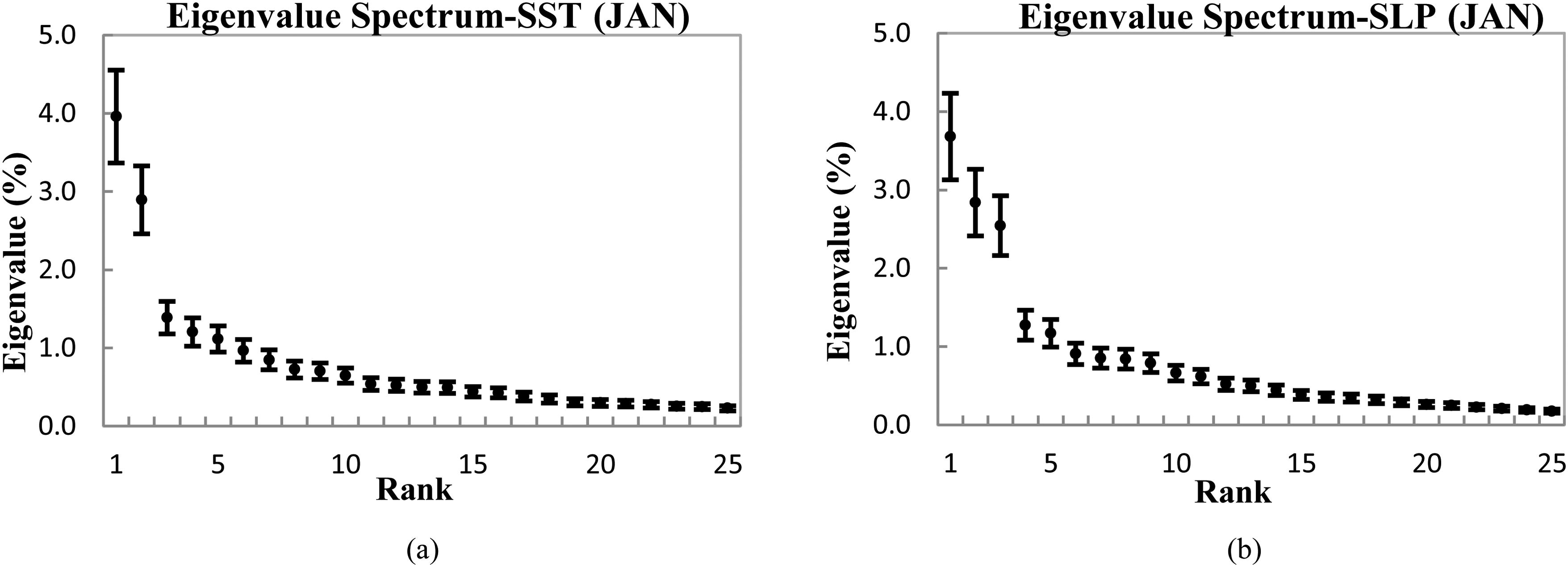
Fig. 2.
(a) Eigenvalue spectrum (%) of the covariance matrix of January SST. The vertical bar shows uncertainty estimates based on North et al. (1982) rule of thumb. The leading 25 eigenvalues out of 41 are shown. (b) Eigenvalue spectrum (%) of the covariance matrix of January SLP. The vertical bar shows uncertainty estimates based on North et al. (1982) rule of thumb. The leading 25 eigenvalues out of 41 are shown.
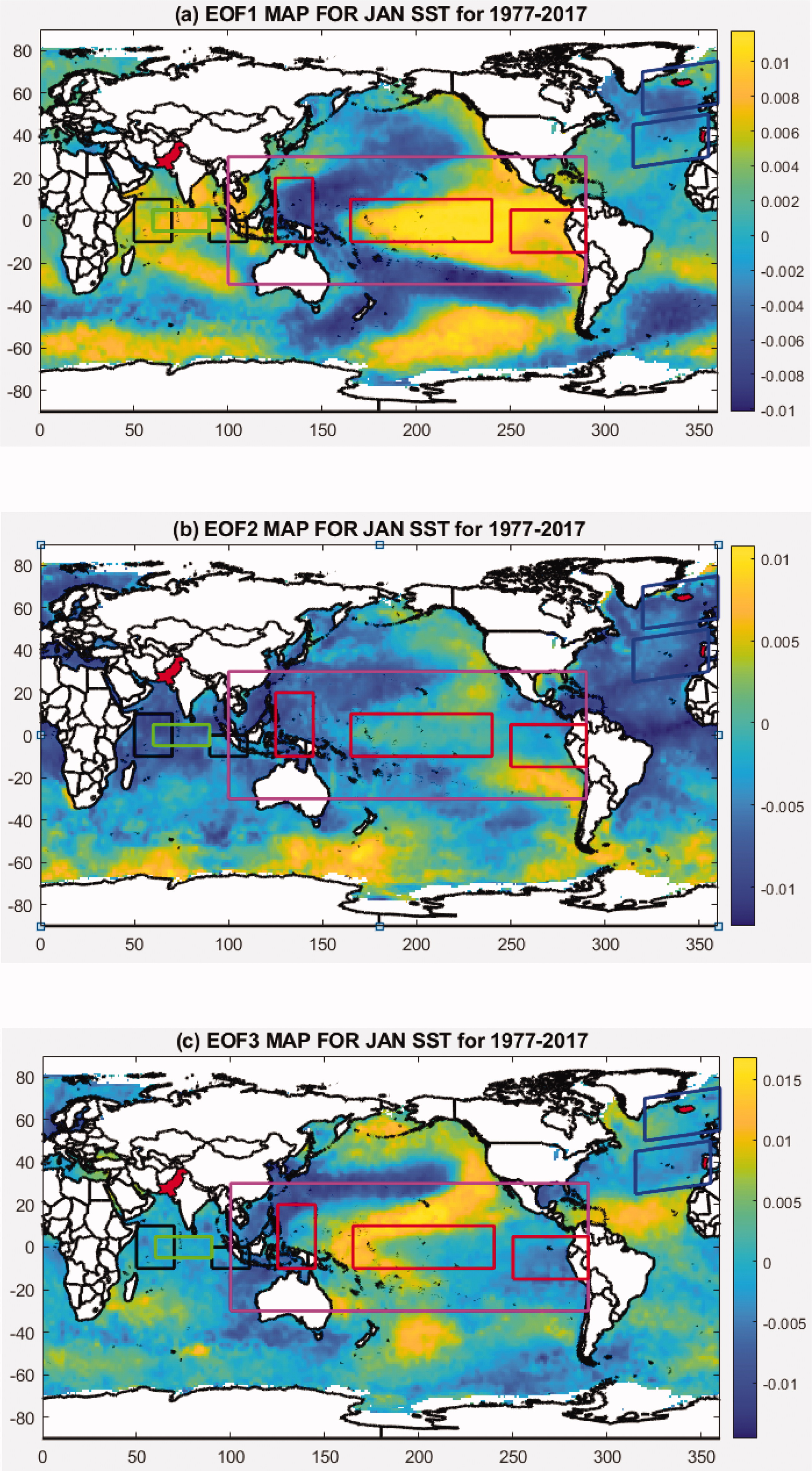
Fig. 3.
EOFs of standardized SST for January over 1977–2017. (a) EOF1 shows the pattern of ENSO and PDO in Pacific Ocean. (b) EOF2 shows the pattern of AMO in Atlantic Ocean and pattern of DMI in Indian Ocean. (c) EOF3 shows PDO, EMI-MODOKI and NAO (SST associated pattern). Black boxes show Western Equatorial Indian Ocean (WEIO) and Eastern Equatorial Indian Ocean (EEIO) region whereas green box shows Central Equatorial Indian Ocean (CEIO) region in Indian Ocean. Red boxes show ENSO-MODOKI regions whereas magenta box shows ENSO-MEI region in Pacific Ocean. Blue boxes show NAO region in Atlantic Ocean.
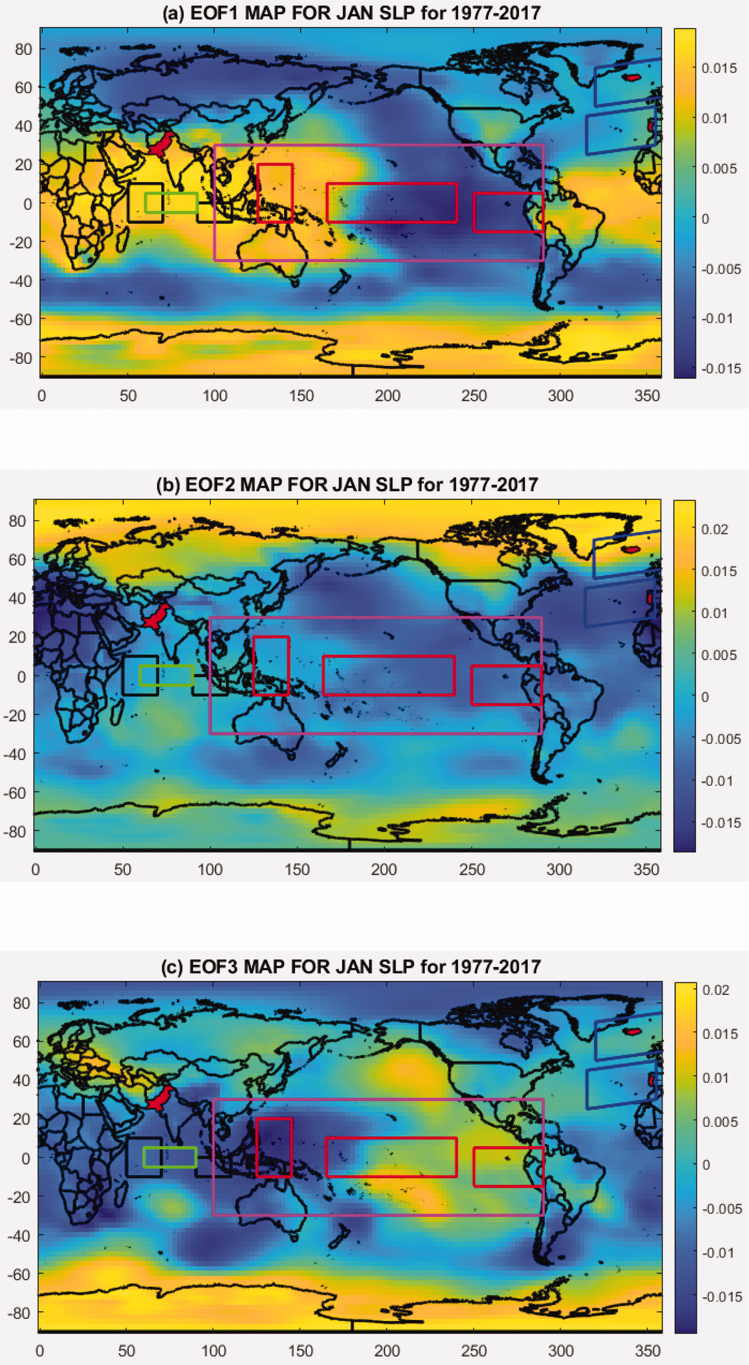
Fig. 4.
EOFs of standardized SLP for January over 1977–2017. (a) EOF1 shows the pattern of ENSO-SOI and NAO pattern though not very distinguished. (b) EOF2 shows the pattern of AO. (c) EOF3 shows patterns of ENSO and NAO pattern though not very distinguished. Black boxes show Western Equatorial Indian Ocean (WEIO) and Eastern Equatorial Indian Ocean (EEIO) region whereas green box shows Central Equatorial Indian Ocean (CEIO) region in Indian Ocean. Red boxes show ENSO-MODOKI regions whereas magenta box shows ENSO-MEI region in Pacific Ocean. Blue boxes show NAO region in Atlantic Ocean.
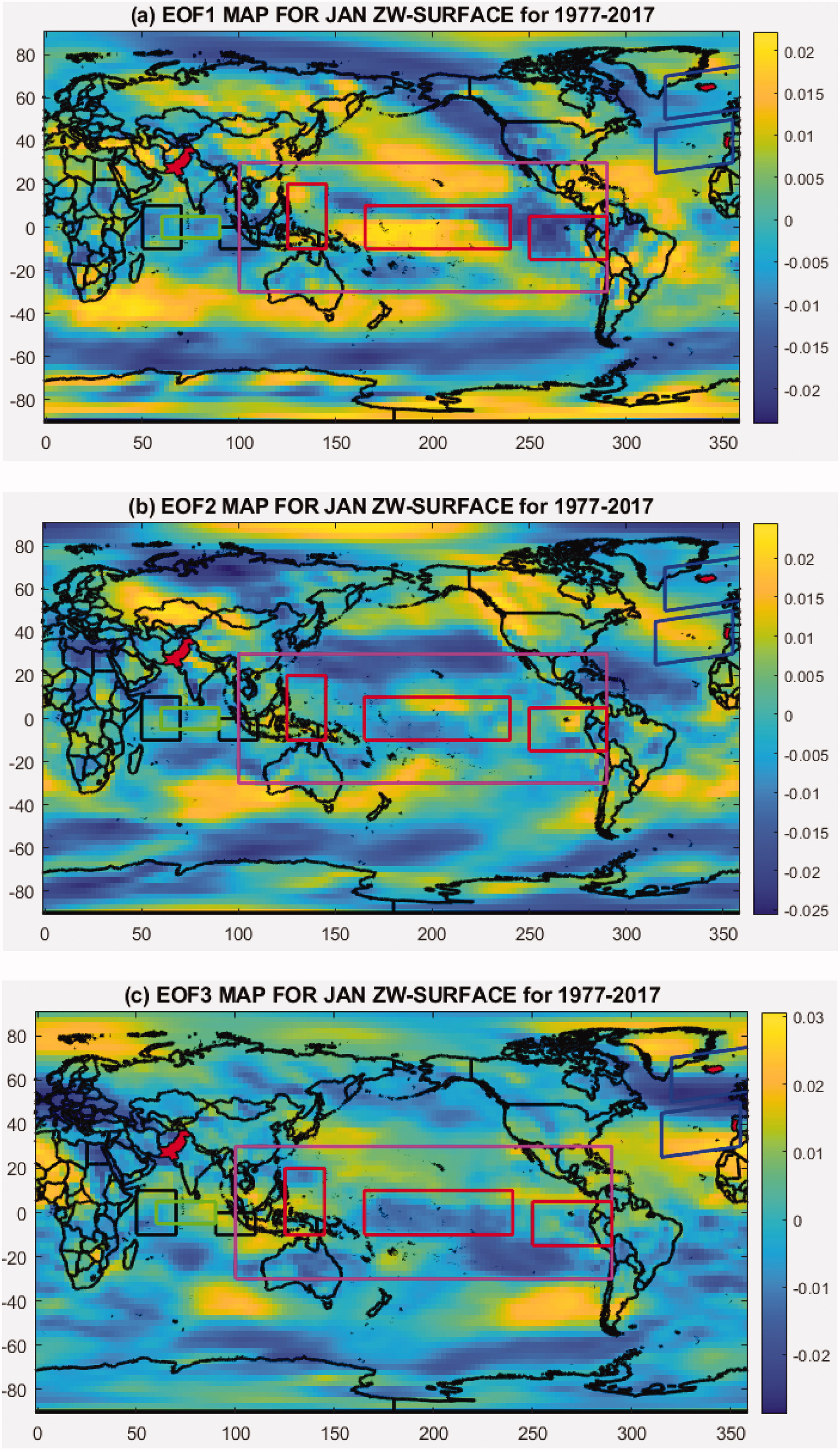
Fig. 5.
EOFs of standardized SZW for January over 1977–2017. (a) EOF1 shows weak patterns of EQWIN. (b) EOF2 shows moderate pattern of EQWIN whereas (c) EOF3 shows weak patterns of EQWIN. Black boxes show Western Equatorial Indian Ocean (WEIO) and Eastern Equatorial Indian Ocean (EEIO) region whereas green box shows Central Equatorial Indian Ocean (CEIO) region in Indian Ocean. Red boxes show ENSO-MODOKI regions whereas magenta box shows ENSO-MEI region in Pacific Ocean. Blue boxes show NAO region in Atlantic Ocean.
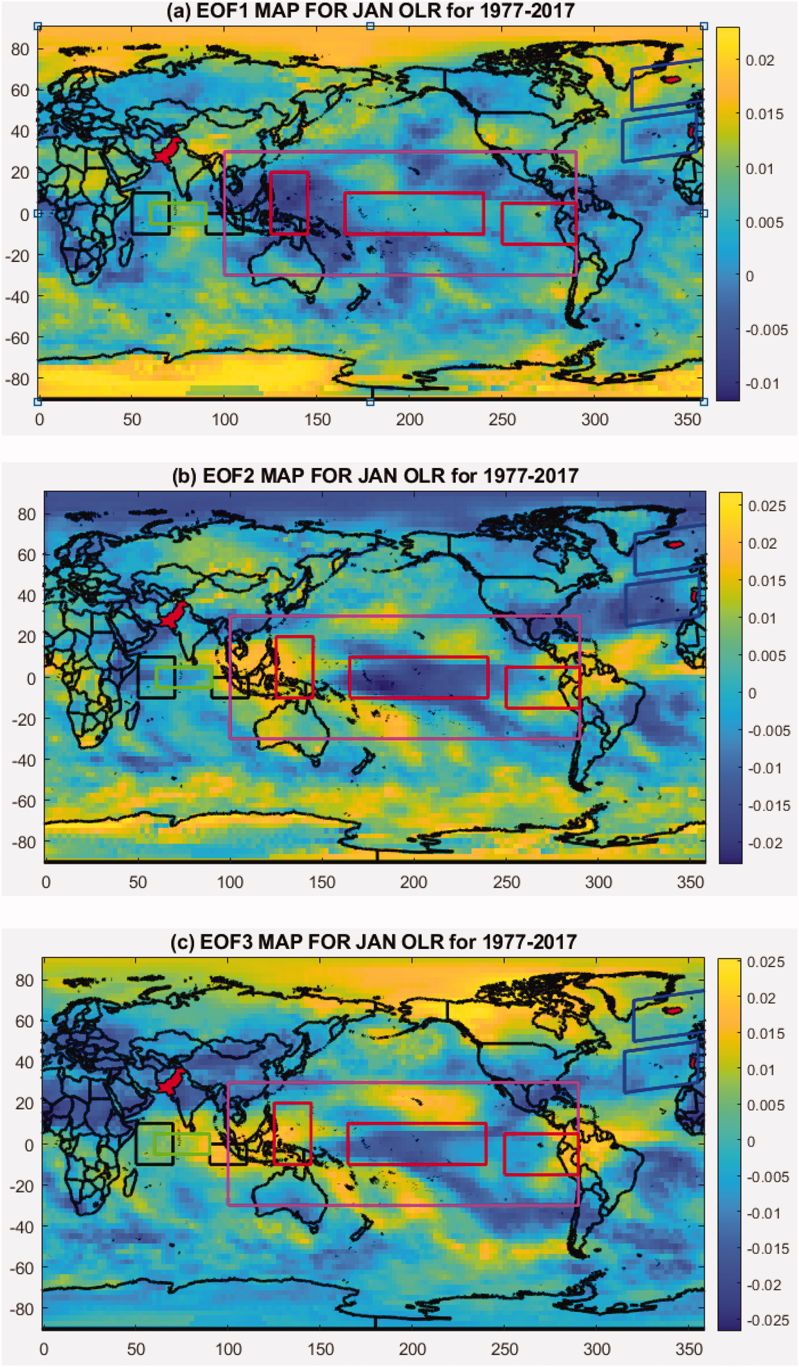
Fig. 6.
EOFs of standardized OLR for January over 1977–2017. (a) EOF1 shows weak patterns of EQUINOO. (b) EOF2 shows moderate pattern of EQUINOO whereas (c) EOF3 shows weak patterns of EQUINOO. Black boxes show Western Equatorial Indian Ocean (WEIO) and Eastern Equatorial Indian Ocean (EEIO) region whereas green box shows Central Equatorial Indian Ocean (CEIO) region in Indian Ocean. Red boxes show ENSO-MODOKI regions whereas magenta box shows ENSO-MEI region in Pacific Ocean. Blue boxes show NAO region in Atlantic Ocean.
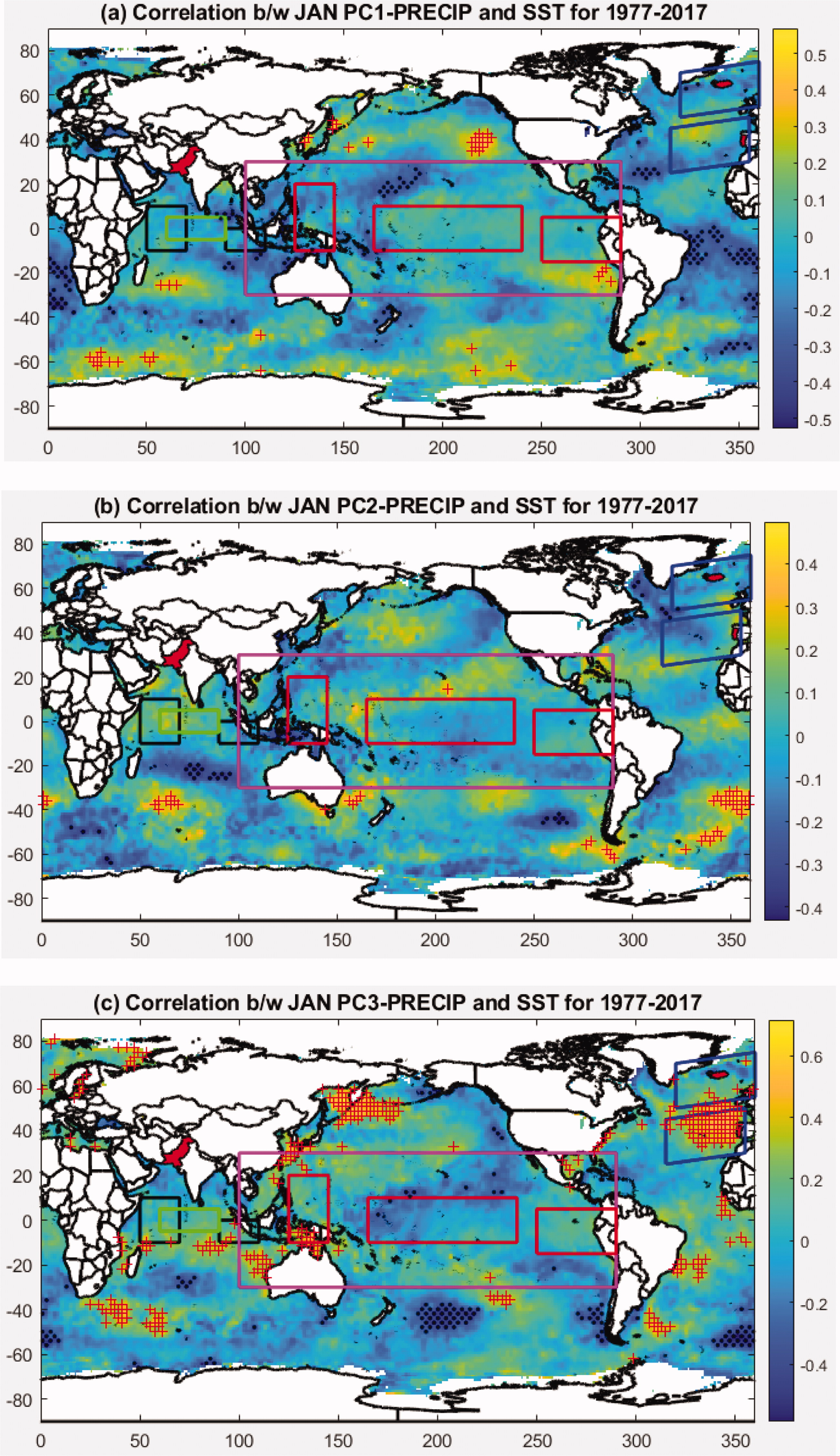
Fig. 7.
Correlation between PCs of Region1 precipitation and standardized SST for January over 1977–2017. (a) PC1 shows weak correlation with DMI. (b) PC2 shows moderate correlation with DMI and weak correlation with EMI-MODOKI. (c) PC3 shows weak correlation with NAO and DMI, moderate correlation with AMO, EMI-MODOKI and PDO. Black boxes show Western Equatorial Indian Ocean (WEIO) and Eastern Equatorial Indian Ocean (EEIO) region whereas green box shows Central Equatorial Indian Ocean (CEIO) region in Indian Ocean. Red boxes show ENSO-MODOKI regions whereas magenta box shows ENSO-MEI region in Pacific Ocean. Blue boxes show NAO region in Atlantic Ocean.
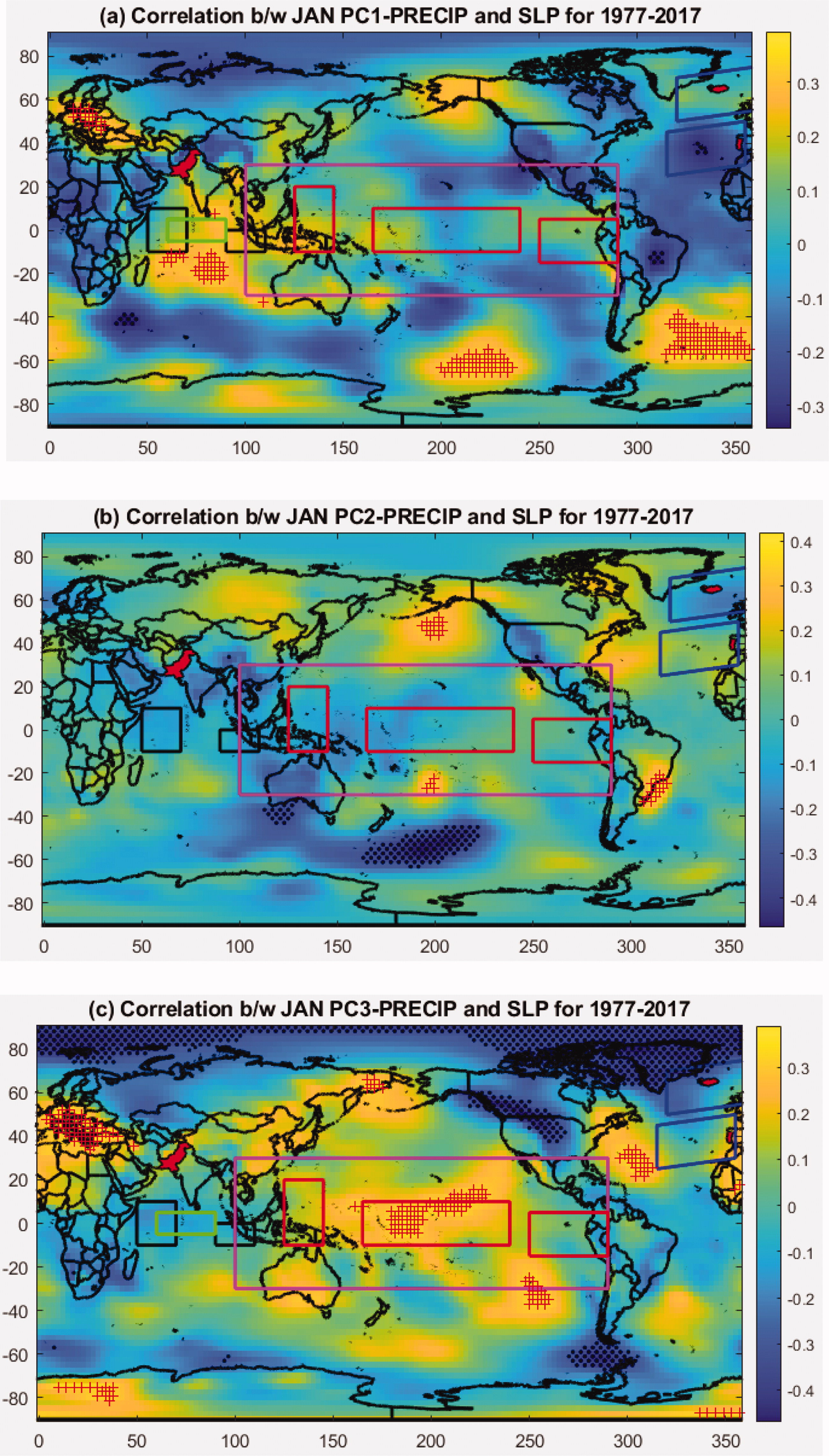
Fig. 8.
Correlation between PCs of Region1 precipitation and standardized SLP for January over 1977–2017. (a) PC1 with SLP. (b) PC2 with SLP. (c) PC3 with SLP. Black boxes show Western Equatorial Indian Ocean (WEIO) and Eastern Equatorial Indian Ocean (EEIO) region whereas green box shows Central Equatorial Indian Ocean (CEIO) region in Indian Ocean. Red boxes show ENSO-MODOKI regions whereas magenta box shows ENSO-MEI region in Pacific Ocean. Blue boxes show NAO region in Atlantic Ocean. Red ‘+’ and Black ‘.’ stipples show significant positive and negative correlation at 5% confidence, respectively.
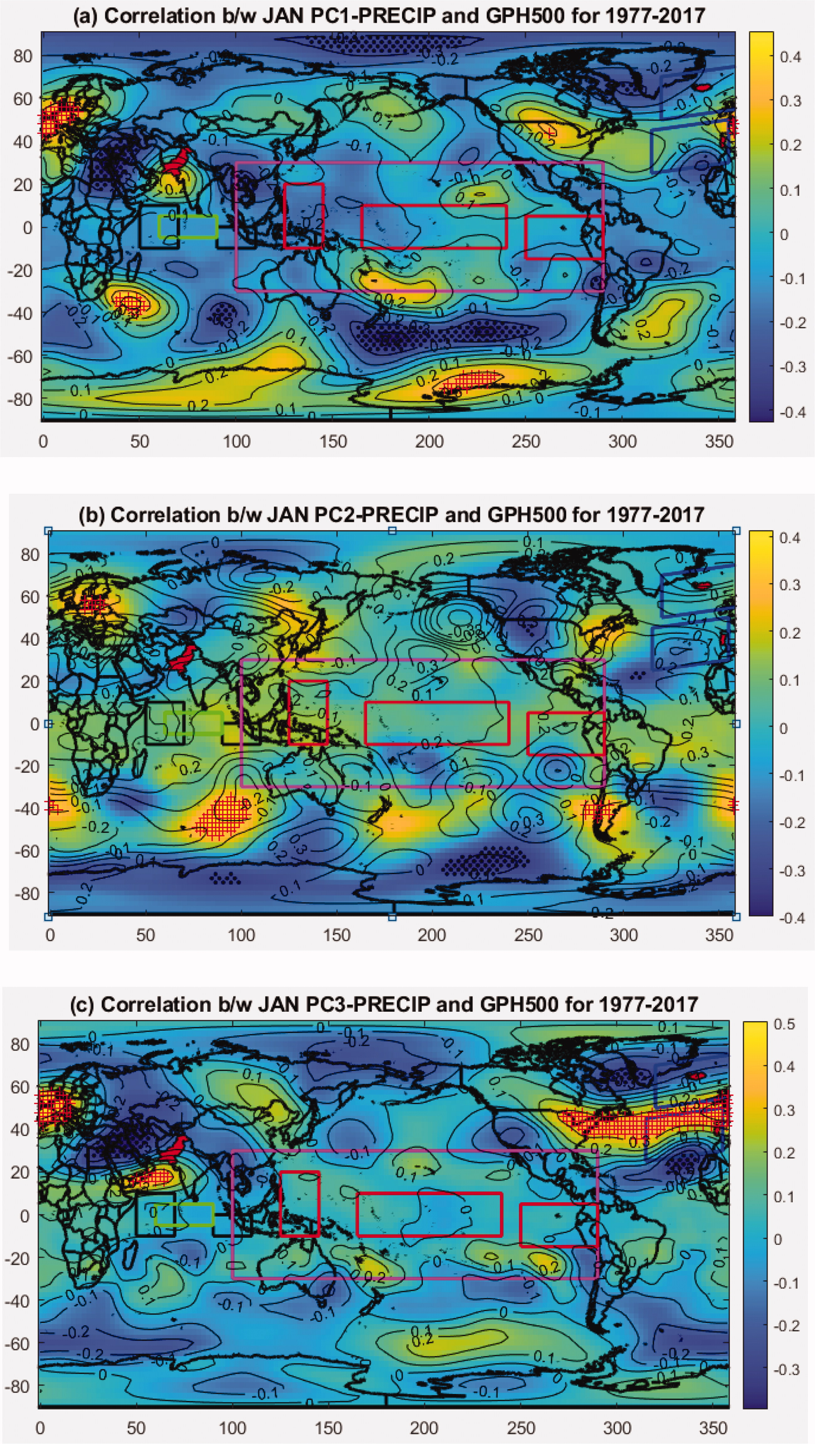
Fig. 9.
Correlation between PCs of Region1 precipitation and standardized GPH500 for January over 1977–2017. (a) PC1 with GPH500. (b) PC2 with GPH500. (c) PC3 with GPH500. Black boxes show Western Equatorial Indian Ocean (WEIO) and Eastern Equatorial Indian Ocean (EEIO) regions. Black boxes show WEIO and EEIO region whereas green box shows Central Equatorial Indian Ocean (CEIO) region in Indian Ocean. Red boxes show ENSO-MODOKI regions whereas magenta box shows ENSO-MEI region in Pacific Ocean. Blue boxes show NAO region in Atlantic Ocean. Red ‘+’ and Black ‘.’ stipples show significant positive and negative correlation at 5% confidence, respectively.
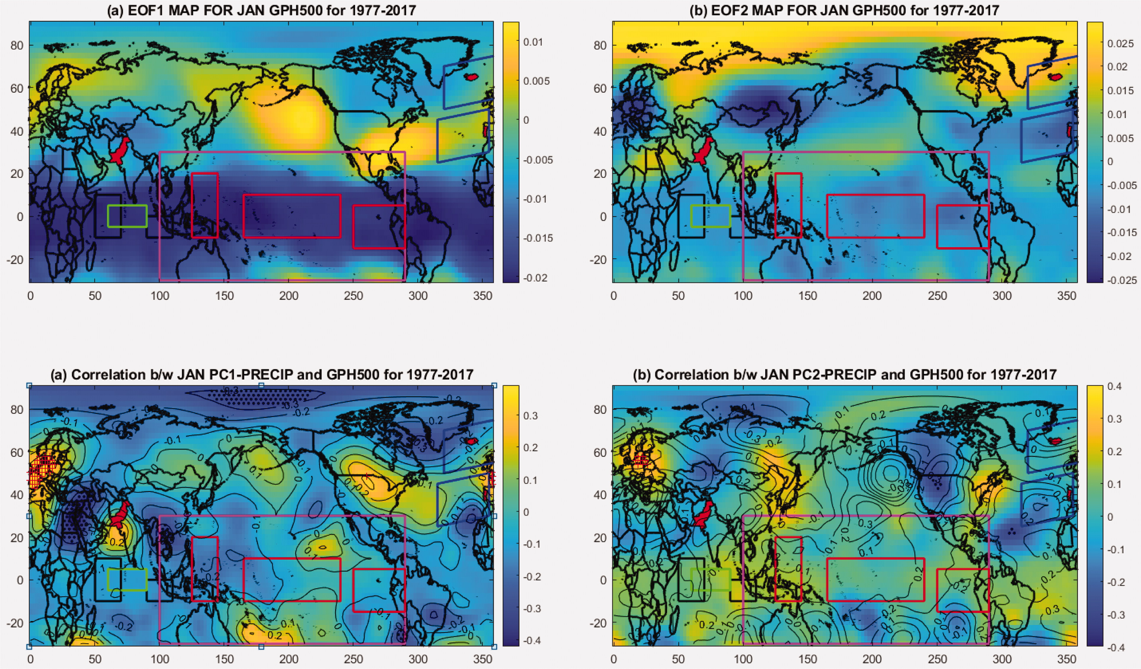
Fig. 10.
EOF modes of standardized GPH at 500 hpa in January and correlation with PCs of Region1 Precipitation. (a) EOF1 mode of GPH500. (b) EOF2 mode of GPH500. (c) Correlation between PC1 with GPH500. (d) Correlation between PC2 with GPH500. Black boxes show Western Equatorial Indian Ocean (WEIO) and Eastern Equatorial Indian Ocean (EEIO) region whereas green box shows Central Equatorial Indian Ocean (CEIO) region in Indian Ocean. Red boxes show ENSO-MODOKI regions whereas magenta box shows ENSO-MEI region in Pacific Ocean. Blue boxes show NAO region in Atlantic Ocean.
Table 7.
Correlation matrix between PCs of GPH (G1, G2, G3) and PCs of Region1 precipitation (PC1, PC2 and PC3).
Table 8.
Correlation between PCs of GPH (G1, G2, G3) and climate indices.
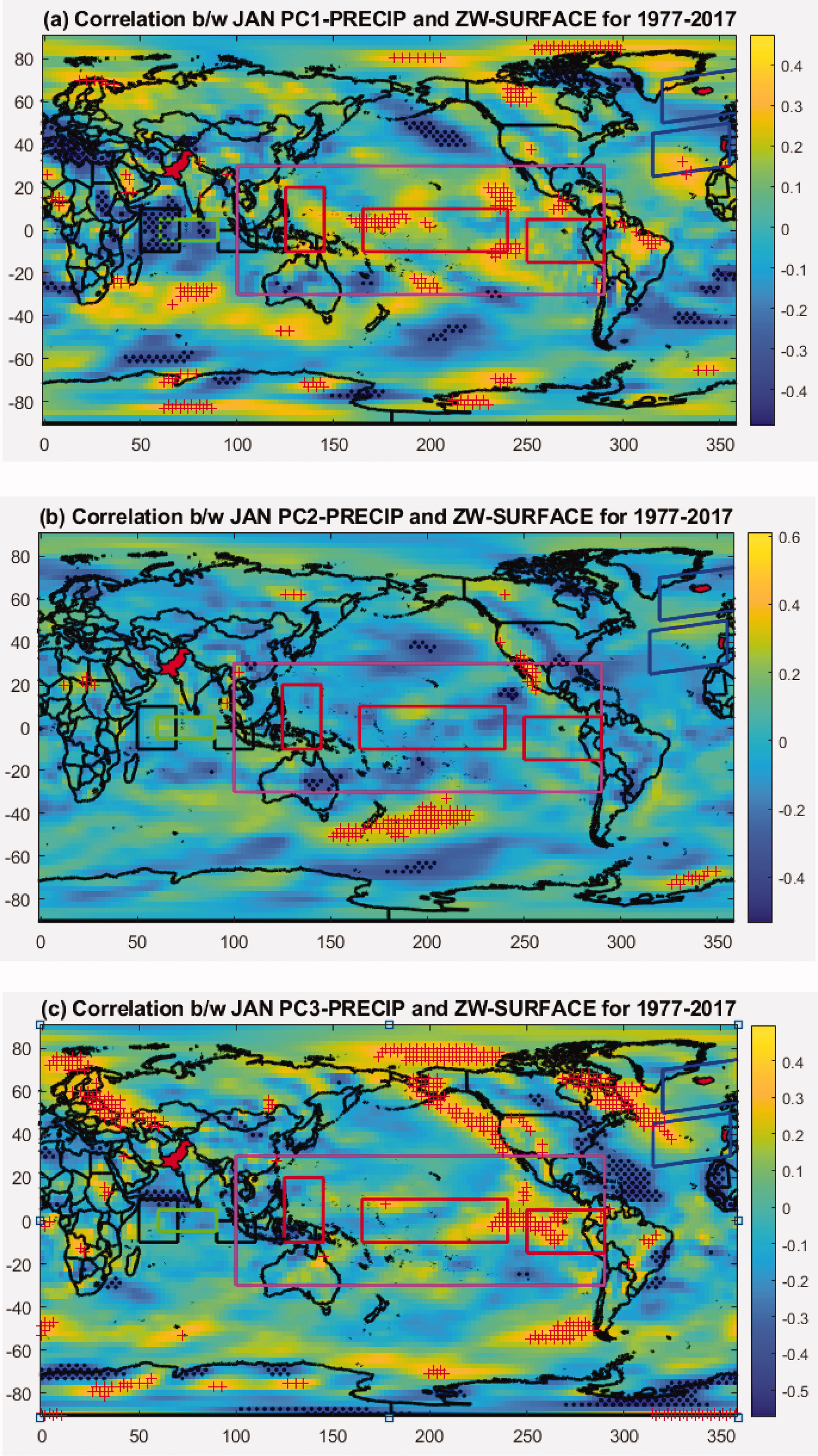
Fig. 11.
PCs of standardized ZW-Surface for January over 1977–2017. (a) PC1 shows strong patterns of EQWIN. (b) PC2 shows weak pattern of EQWIN whereas (c) PC3 shows weak pattern of EQWIN. Black boxes show WEIO and EEIO region whereas green box shows CEIO region in Indian Ocean. Red boxes show ENSO-MODOKI regions whereas magenta box shows ENSO-MEI region in Pacific Ocean. Blue boxes show NAO region in Atlantic Ocean.
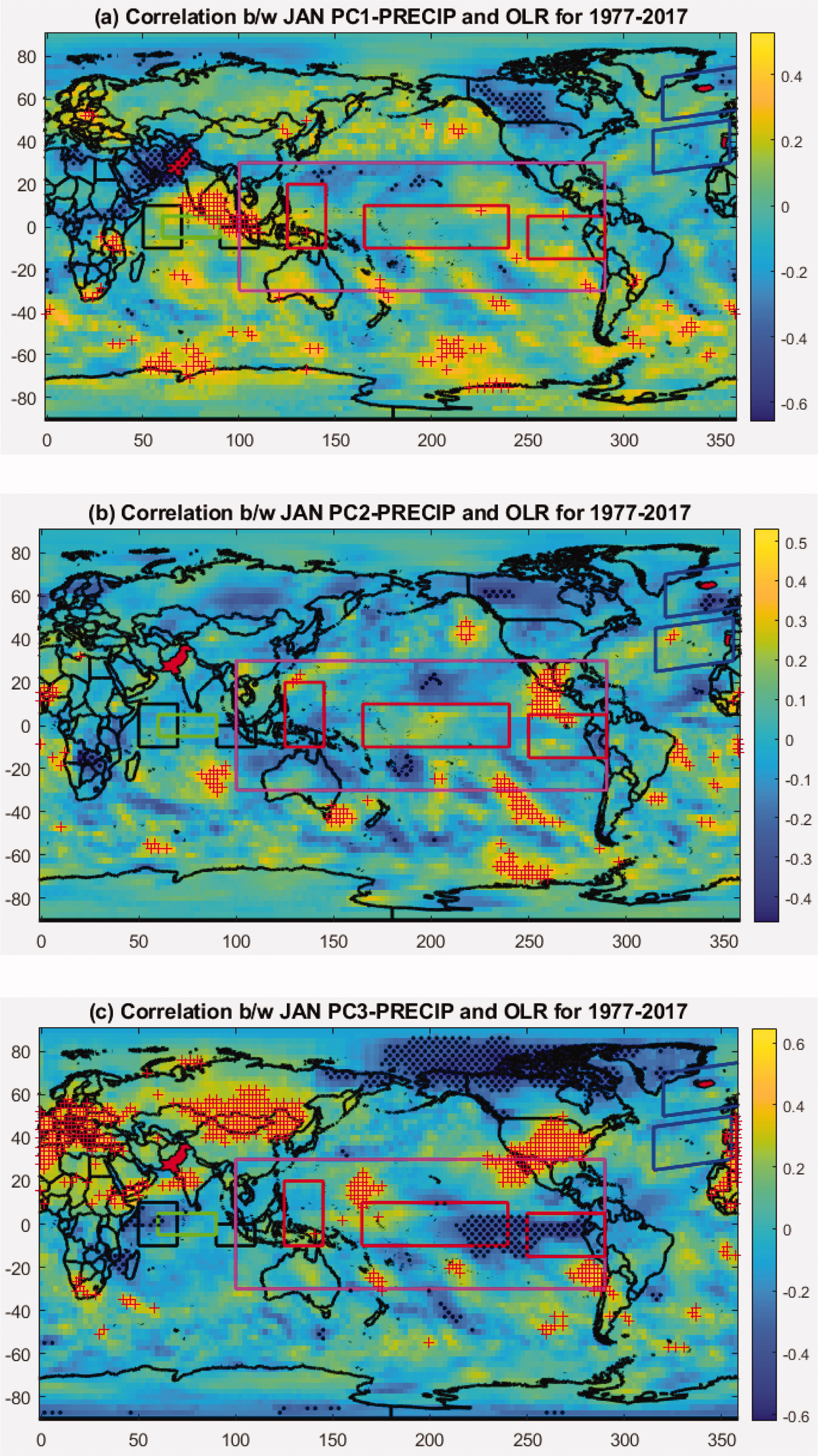
Fig. 12.
EOFs of standardized OLR for January over 1977–2017. (a) EOF1 shows strong patterns of EQWIN. (b) EOF2 shows weak pattern of EQWIN whereas (c) EOF3 shows patterns of EQWIN. Black boxes show WEIO and EEIO region whereas green Box shows CEIO region in Indian Ocean. Red boxes show ENSO-MODOKI regions whereas magenta box shows ENSO-MEI region in Pacific Ocean. Blue boxes show NAO region in Atlantic Ocean.
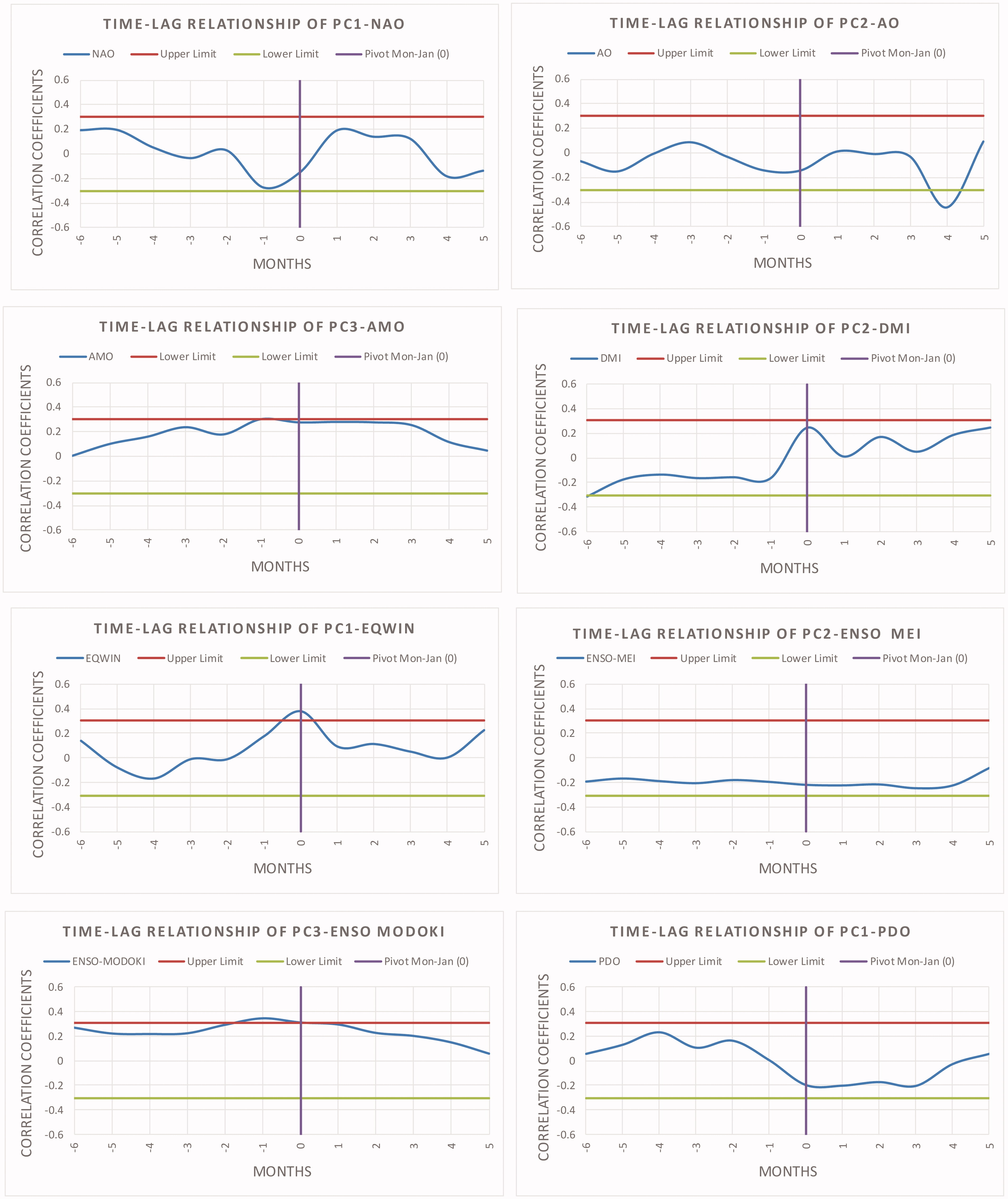
Fig. 13.
Time-lag correlation coefficient between most significant PCs and Climate Indices. January is considered as the pivot month with a value “0” represented by a vertical line whereas negative/positive values along x-axis (Months) indicates preceding/following months from January. Upper and lower limit represents the significance level of 5%.
Table 9.
Summary of analysis results for Region1 precipitation and climate indices for January.
PCs and Climate IndicesEOF analysisCorrelation b/w PCs and anomalies ofSSTAtmospheric circulationZonal winds/OLRNAOWeakInsignificantWeakWeakModerate–AOWeakInsignificantModerate to Weak–Weak–AMOWeakSignificant at 7.9%ModerateModerate––DMIWeakSignificant at 12.4%ModerateModerate––EQWINStrong to ModerateSignificant at 1.5 %Strong––StrongENSO-MEIModerate to WeakSignificant at 16.5 %ModerateWeak––EMI-MODOKIStrongSignificant at 4.8 %StrongStrong––PDOWeakSignificant at 20.5 %ModerateModerate to Strong––
Table 11.
Correlation between R1JANP-PCs and climate indices.
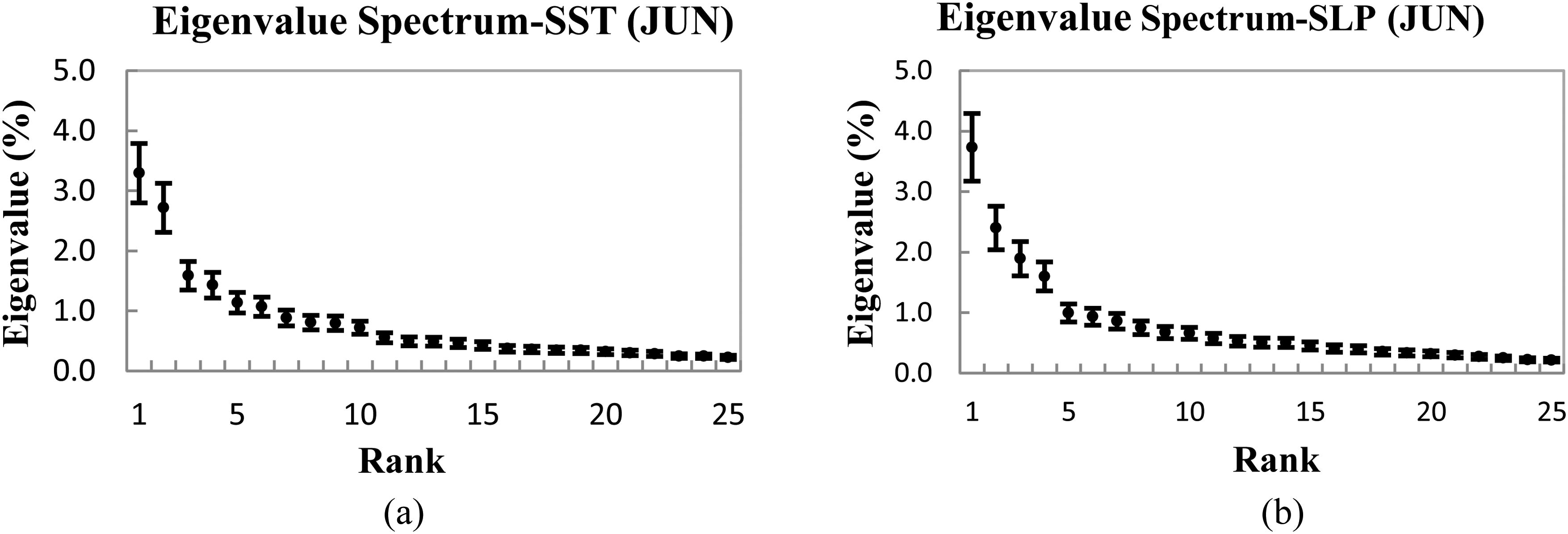
Fig. 14.
(a) Eigenvalue spectrum (%) of the covariance matrix of June SST. The vertical bar shows uncertainty estimates based on North et al. (1982) rule of thumb. The leading 25 eigenvalues out of 41 are shown. (b) Eigenvalue spectrum (%) of the covariance matrix of June SLP. The vertical bar shows uncertainty estimates based on North et al. (1982) rule of thumb. The leading 25 eigenvalues out of 41 are shown.
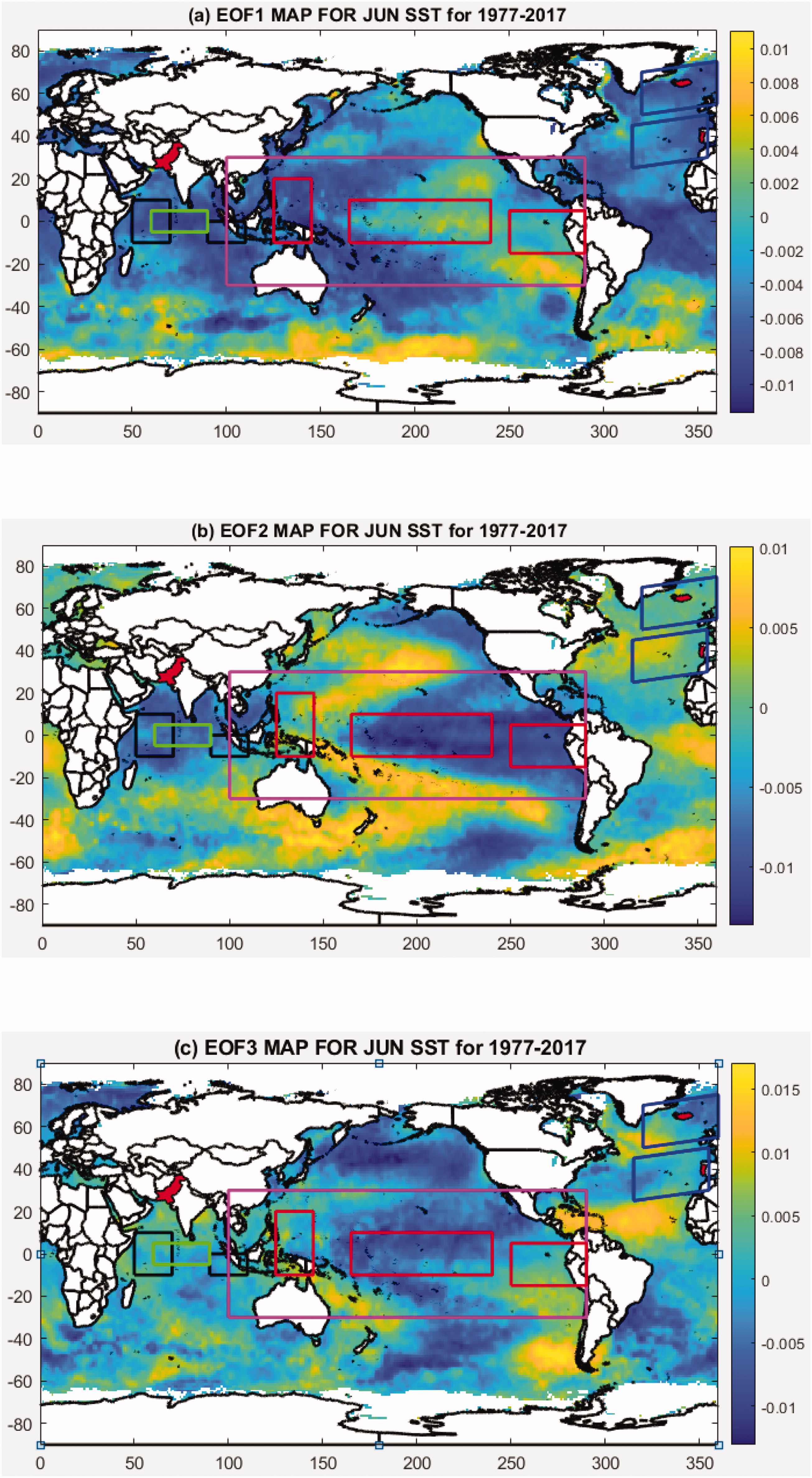
Fig. 15.
EOFs of standardized SST for June over 1977–2017. (a) EOF1 shows the Pattern of EMI-MODOKI in central Pacific Ocean though weak in one of the flank and AMO in North Atlantic Ocean. (b) EOF2 shows the patterns of NAO (associated SST pattern; though weak) in North Atlantic Ocean, ENSO-MEI in central Pacific and PDO in North Pacific. (c) EOF3 shows weak patterns of DMI, EMI-MODOKI and NAO (associated SST pattern). Black boxes show WEIO and EEIO region whereas green Box shows CEIO region in Indian Ocean. Red boxes show ENSO-MODOKI regions whereas magenta box shows ENSO-MEI region in Pacific Ocean. Blue boxes show NAO region in Atlantic Ocean.
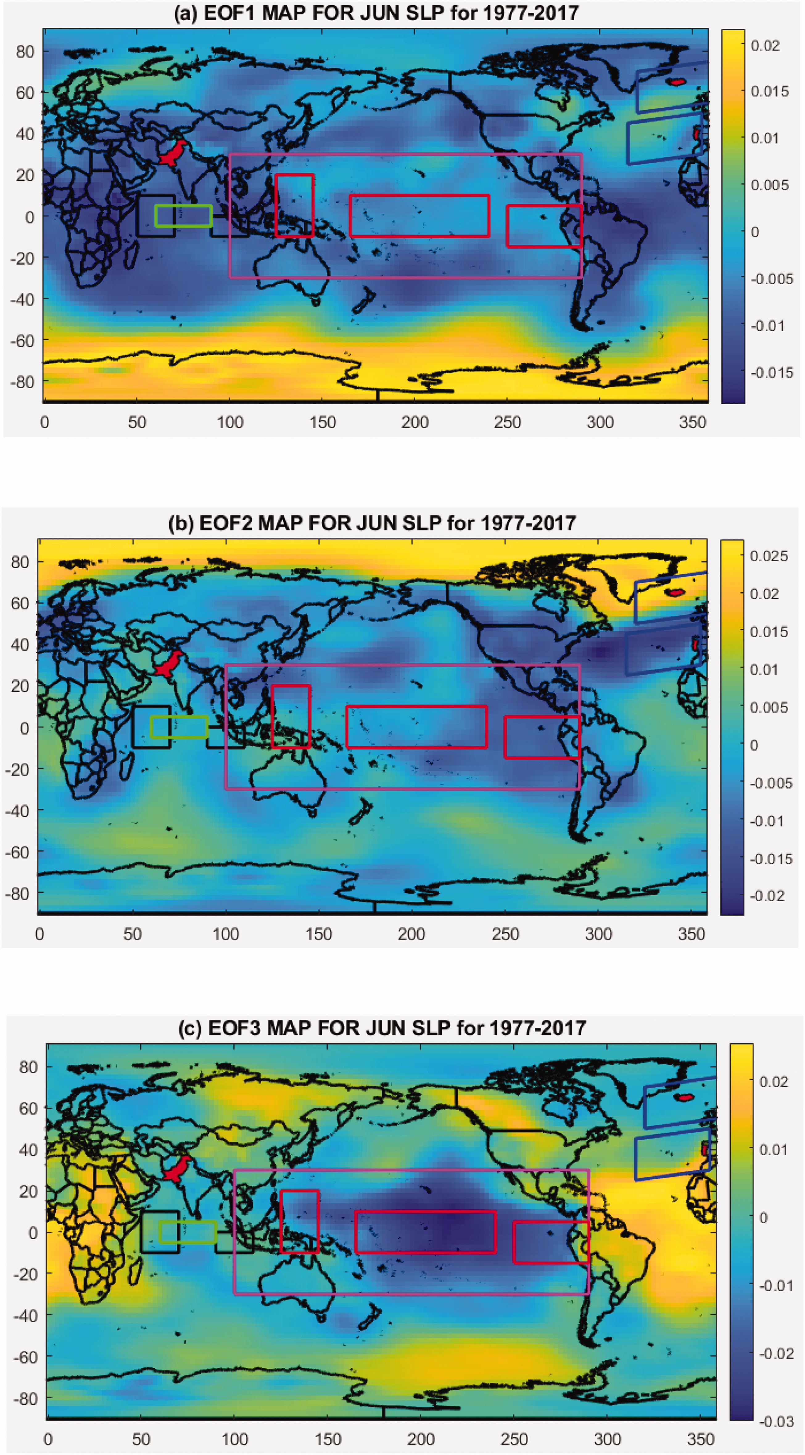
Fig. 16.
EOFs of standardized SLP for June over 1977–2017. (a) EOF1 shows the Pattern of NAO though not very distinguished. (b) EOF2 shows the pattern of NAO. (c) EOF3 shows patterns of ENSO-MEI and AO though not very distinguished. Black boxes show WEIO and EEIO region whereas green box shows CEIO region in Indian Ocean. Red boxes show ENSO-MODOKI regions whereas magenta box shows ENSO-MEI region in Pacific Ocean. Blue boxes show NAO region in Atlantic Ocean.
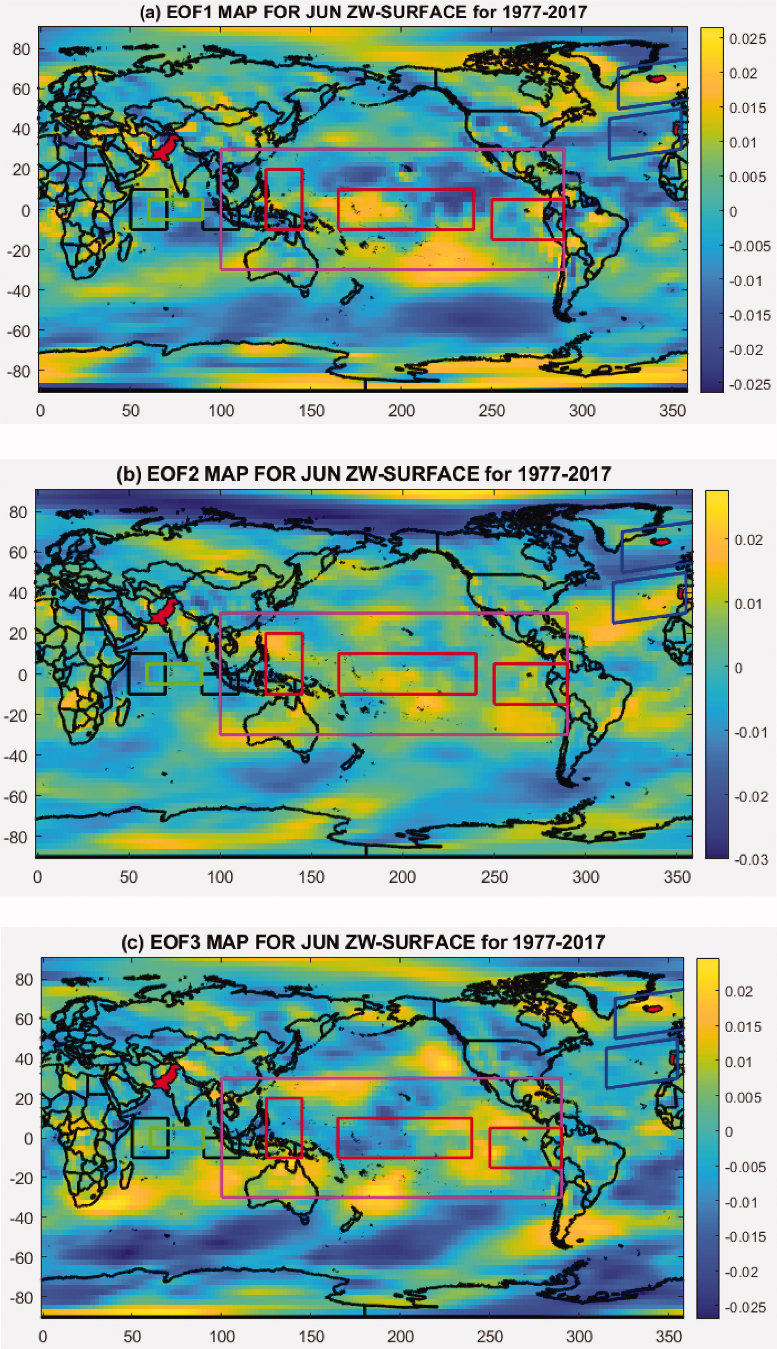
Fig. 17.
EOFs of standardized ZW-surface for June over 1977–2017. (a) EOF1 shows weak patterns of EQWIN. (b) EOF2 shows weak pattern of EQWIN whereas (c) EOF3 shows patterns of EQWIN. Black boxes show WEIO and EEIO region whereas green box shows CEIO region in Indian Ocean. Red boxes show ENSO-MODOKI regions whereas magenta box shows ENSO-MEI region in Pacific Ocean. Blue boxes show NAO region in Atlantic Ocean.
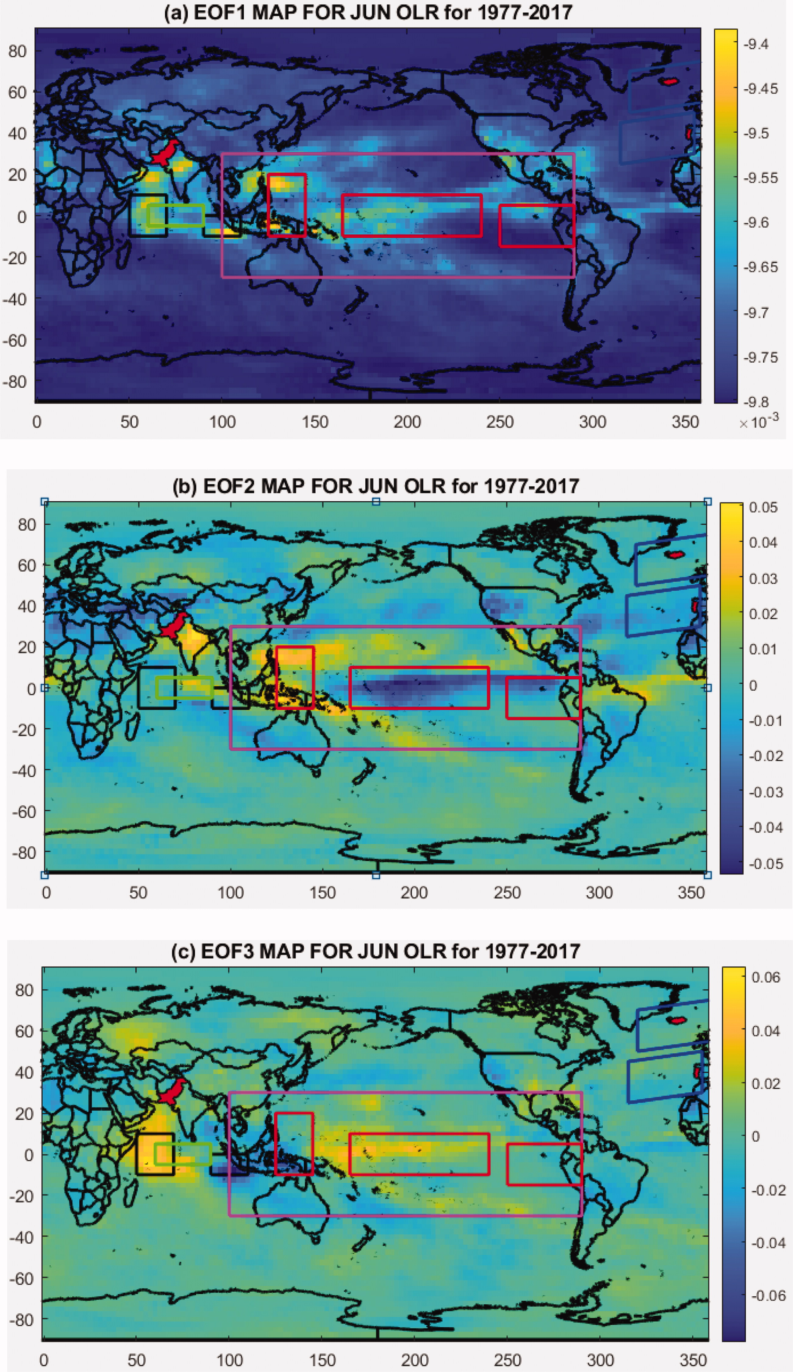
Fig. 18.
EOFs of standardized OLR for June over 1977–2017. (a) EOF1 shows weak patterns of EQUINOO. (b) EOF2 shows weak pattern of EQUINOO whereas (c) EOF3 shows moderate patterns of EQUINOO. Black boxes show WEIO and EEIO region whereas green box shows CEIO region in Indian Ocean. Red boxes show ENSO-MODOKI regions whereas magenta box shows ENSO-MEI region in Pacific Ocean. Blue boxes show NAO region in Atlantic Ocean.
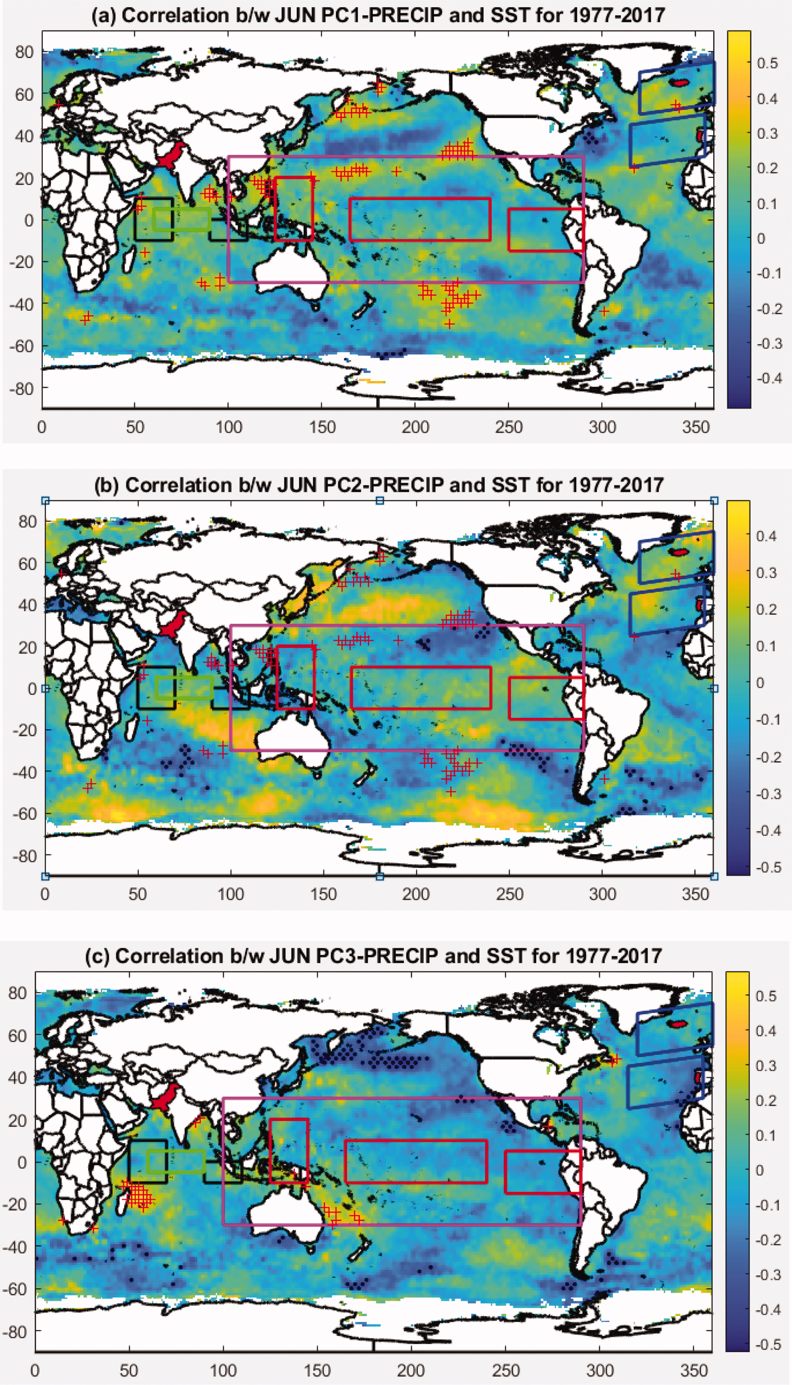
Fig. 19.
Correlation between PCs of Region1 precipitation and standardized SST for June over 1977–2017. (a) PC1 shows weak correlation with NAO (associated SST pattern) and ENSO-MEI whereas moderate correlation with PDO. (b) PC2 shows weak correlation with EMI-MODOKI and string correlation with PDO. (c) PC3 shows weak correlation with DMI and ENSO-MEI but moderate correlation with AMO. Black boxes show WEIO and EEIO region whereas green box shows CEIO region in Indian Ocean. Red boxes show ENSO-MODOKI regions whereas magenta box shows ENSO-MEI region in Pacific Ocean. Blue boxes show NAO region in Atlantic Ocean.
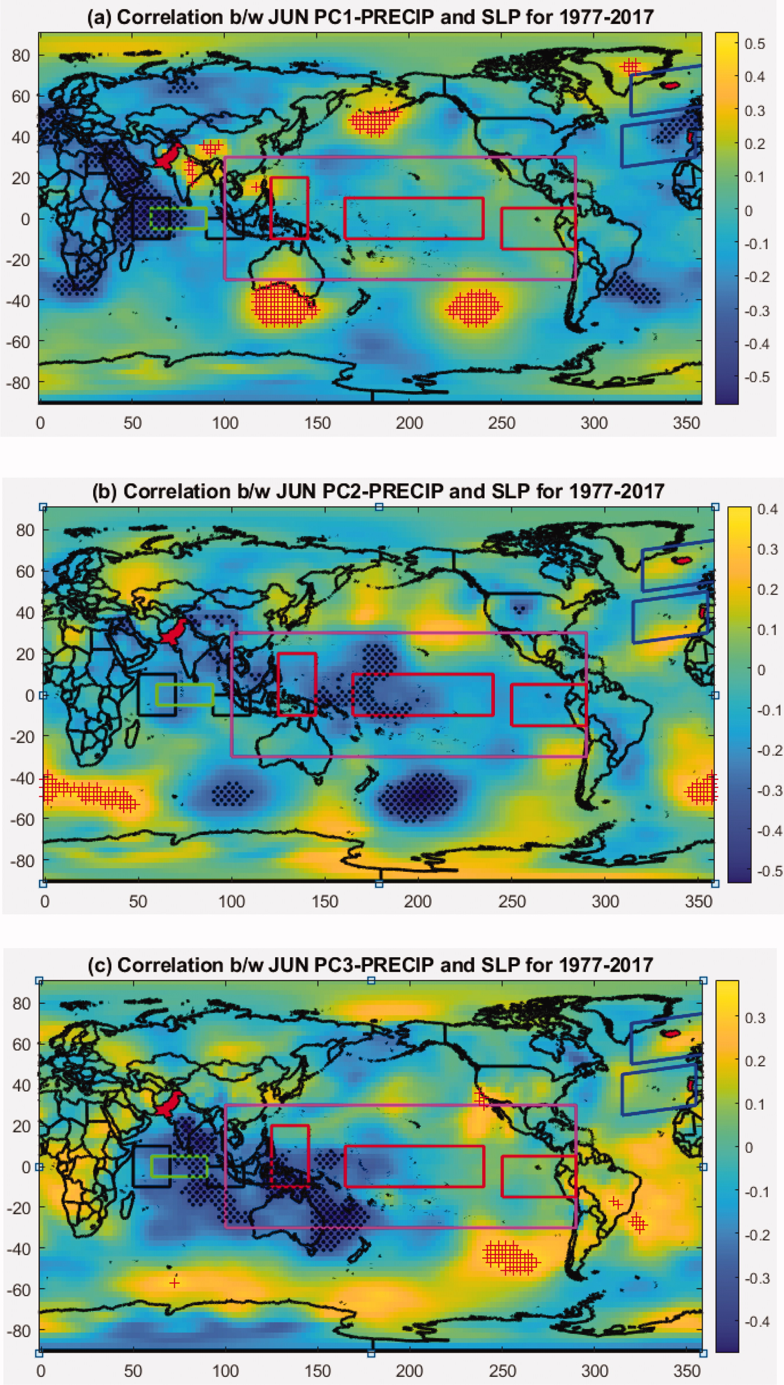
Fig. 20.
Correlation between PCs of Region1 precipitation and standardized SLP for June over 1977–2017. (a) PC1 with SLP. (b) PC2 with SLP. (c) PC3 with SLP. Black boxes show WEIO and EEIO regions. Black boxes show WEIO and EEIO region whereas green box shows CEIO region in Indian Ocean. Red boxes show ENSO-MODOKI regions whereas magenta box shows ENSO-MEI region in Pacific Ocean. Blue boxes show NAO region in Atlantic Ocean. Red ‘+’ and Black ‘.’ stipples show significant positive and negative correlation at 5% confidence, respectively.
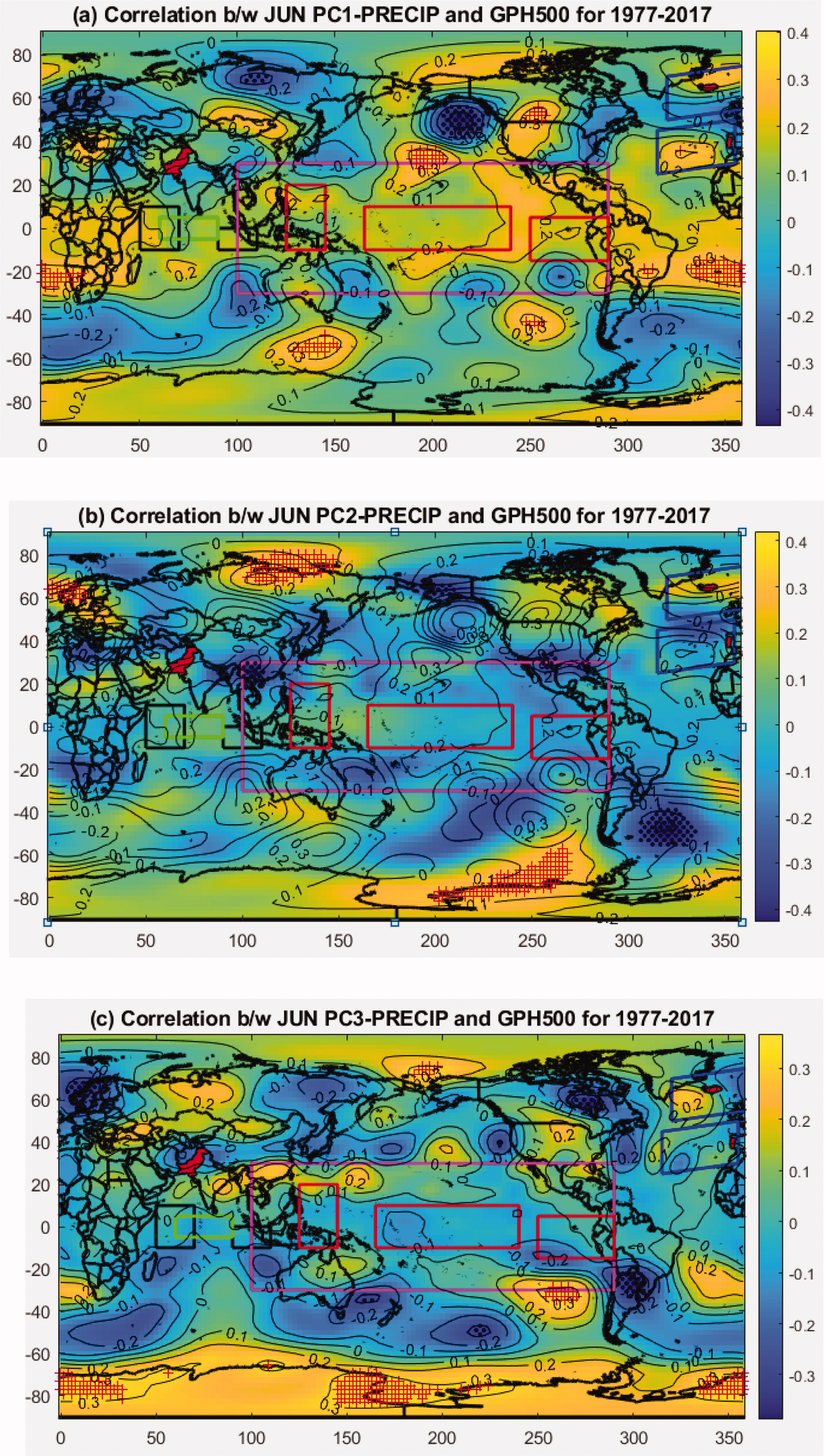
Fig. 21.
Correlation between PCs of Region1 precipitation and standardized GPH500 for June over 1977–2017. (a) PC1 with GPH500. (b) PC2 with GPH500. (c) PC3 with GPH500. Black boxes show WEIO and EEIO regions. Black boxes show WEIO and EEIO region whereas green box shows CEIO region in Indian Ocean. Red boxes show ENSO-MODOKI regions whereas magenta box shows ENSO-MEI region in Pacific Ocean. Blue boxes show NAO region in Atlantic Ocean. Red ‘+’ and Black ‘.’ stipples show significant positive and negative correlation at 5% confidence, respectively.
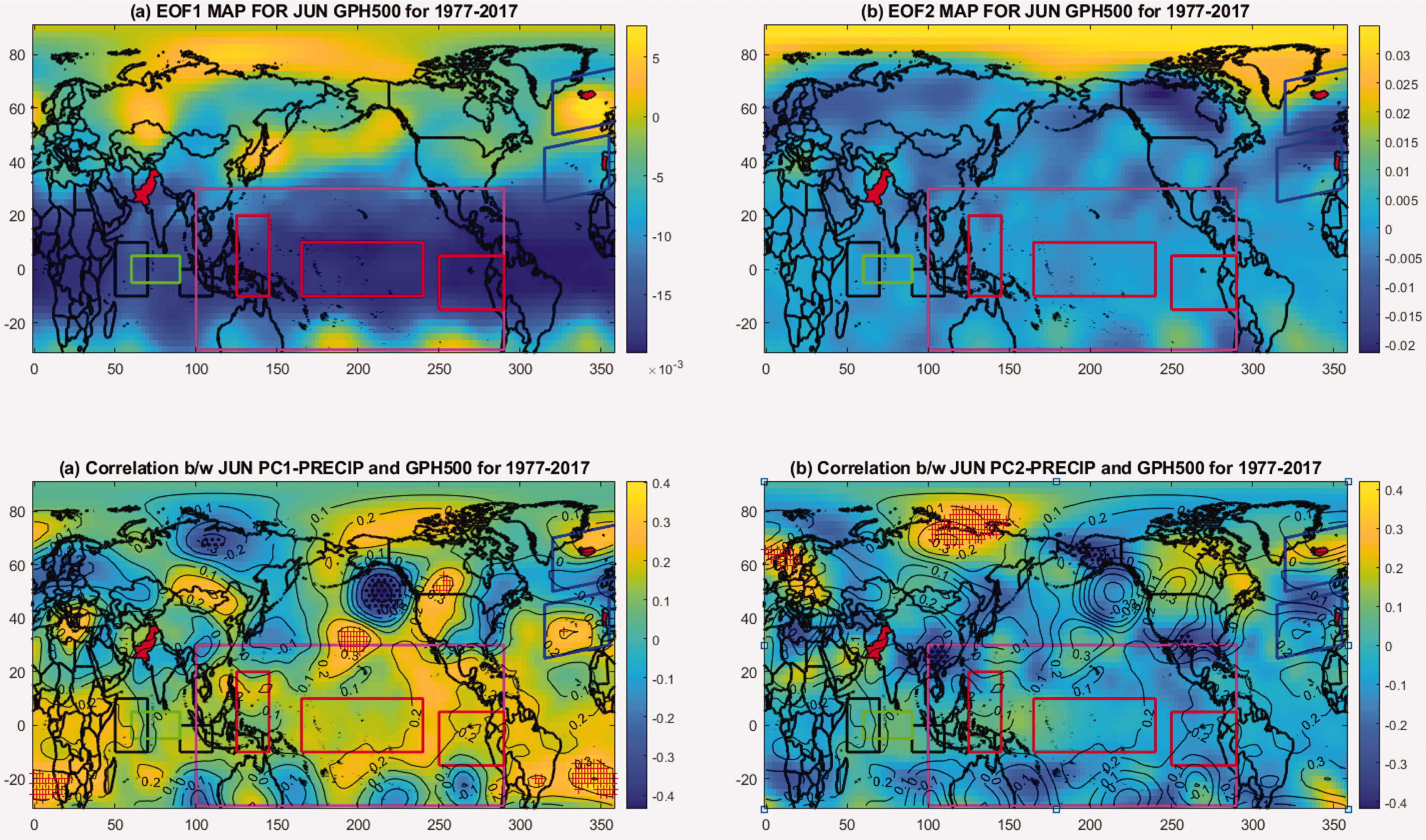
Fig. 22.
EOF modes of standardized GPH at 500 hpa in June and correlation with PCs of Region1 precipitation. (a) EOF1 mode of GPH500. (b) EOF2 mode of GPH500. (c) Correlation between PC1 with GPH500. (d) Correlation between PC2 with GPH500. Black boxes show WEIO and EEIO regions. Red boxes show ENSO-MODOKI Regions and Magenta box shows ENSO-MEI Region. Blue boxes show NAO region. Red ‘+’ and Black ‘.’ stipples show significant positive and negative correlation at 5% confidence, respectively.
Table 12.
Correlation matrix of p-value between PCs of GPH (G1, G2, G3) and PCs of Region1 precipitation (PC1, PC2 and PC3).
Table 13.
Correlation between PCs of GPH (G1, G2, G3) and climate indices.
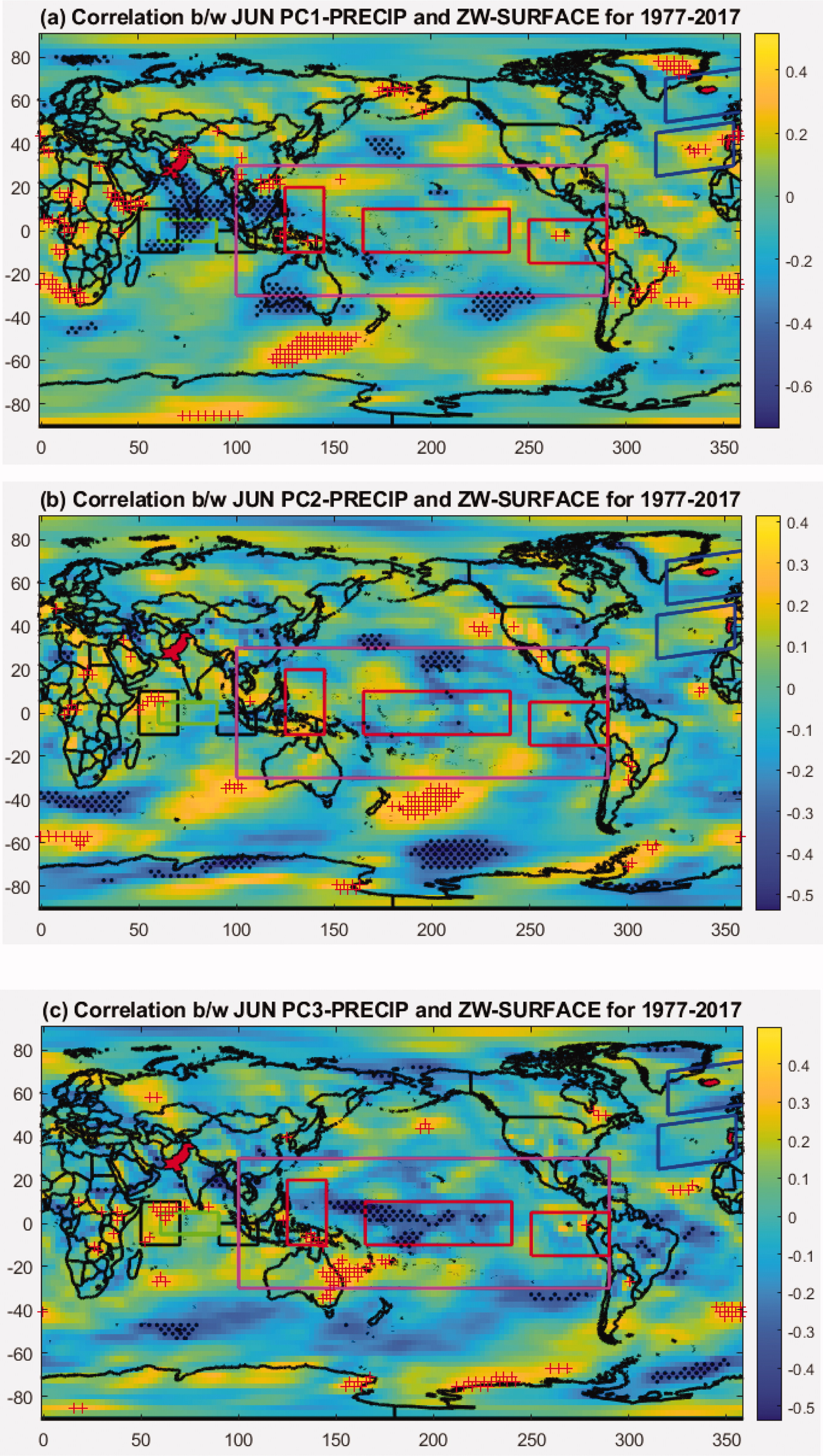
Fig. 23.
EOFs of standardized ZW-surface for June over 1977–2017. (a) EOF1 shows strong patterns of EQWIN. (b) EOF2 shows weak pattern of EQWIN whereas (c) EOF3 shows strong pattern of EQWIN. Blue box shows WEIO region and red box shows EEIO region. Black boxes show WEIO and EEIO region whereas green box shows CEIO region in Indian Ocean. Red boxes show ENSO-MODOKI regions whereas magenta box shows ENSO-MEI region in Pacific Ocean. Blue boxes show NAO region in Atlantic Ocean. Red ‘+’ and Black ‘.’ stipples show significant negative and positive correlation at 5% confidence respectively.
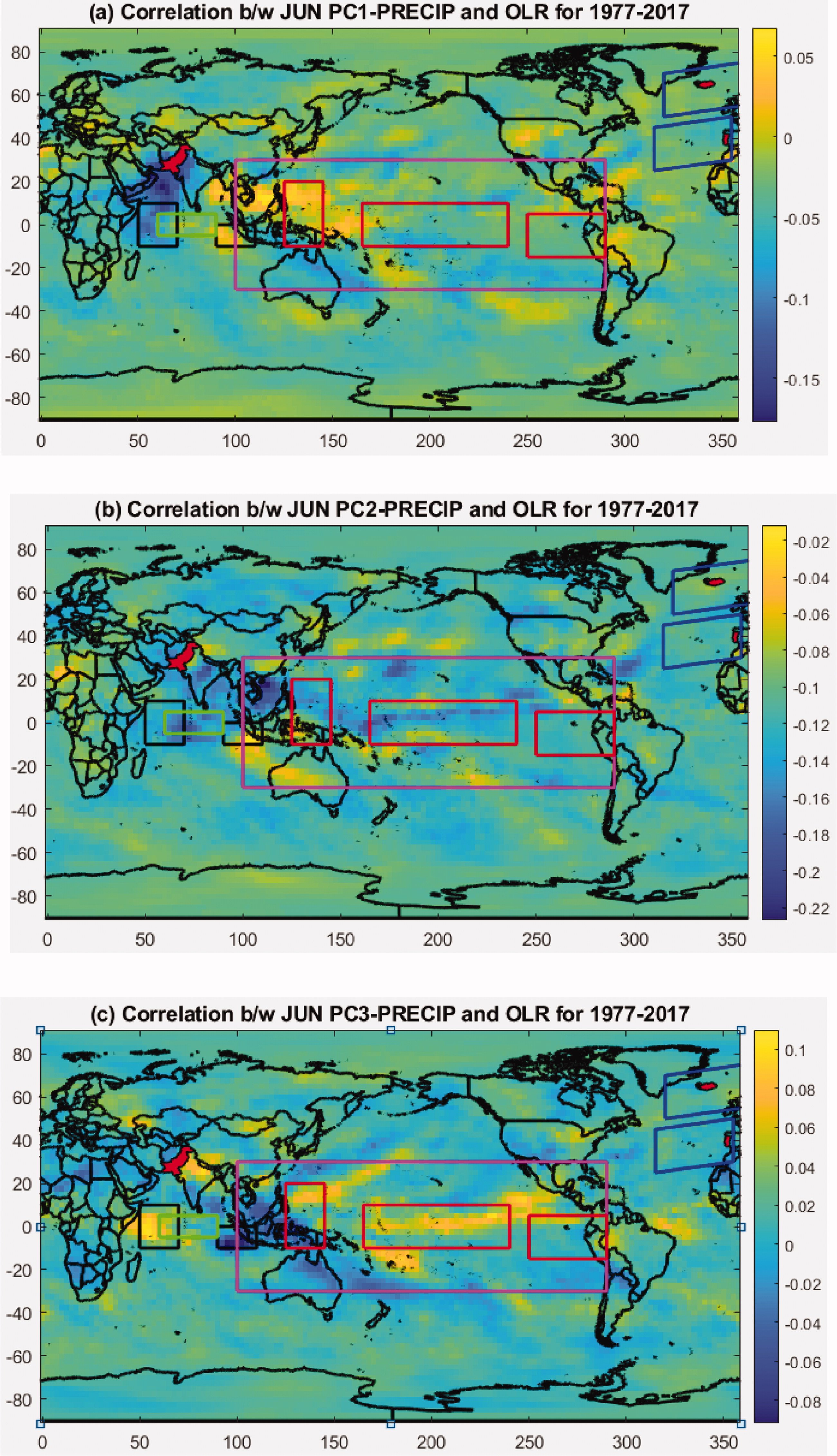
Fig. 24.
EOFs of standardized ZW-surface for June over 1977–2017. (a) EOF1 shows moderate patterns of EQUINOO. (b) EOF2 shows weak pattern of EQUINOO whereas (c) EOF3 shows moderate pattern of EQUINOO. Blue box shows WEIO region and red box shows EEIO region. Black boxes show WEIO and EEIO region whereas green box shows CEIO region in Indian Ocean. Red boxes show ENSO-MODOKI regions whereas magenta box shows ENSO-MEI region in Pacific Ocean. Blue boxes show NAO region in Atlantic Ocean. Red ‘+’ and Black ‘.’ stipples show significant negative and positive correlation at 5% confidence respectively.
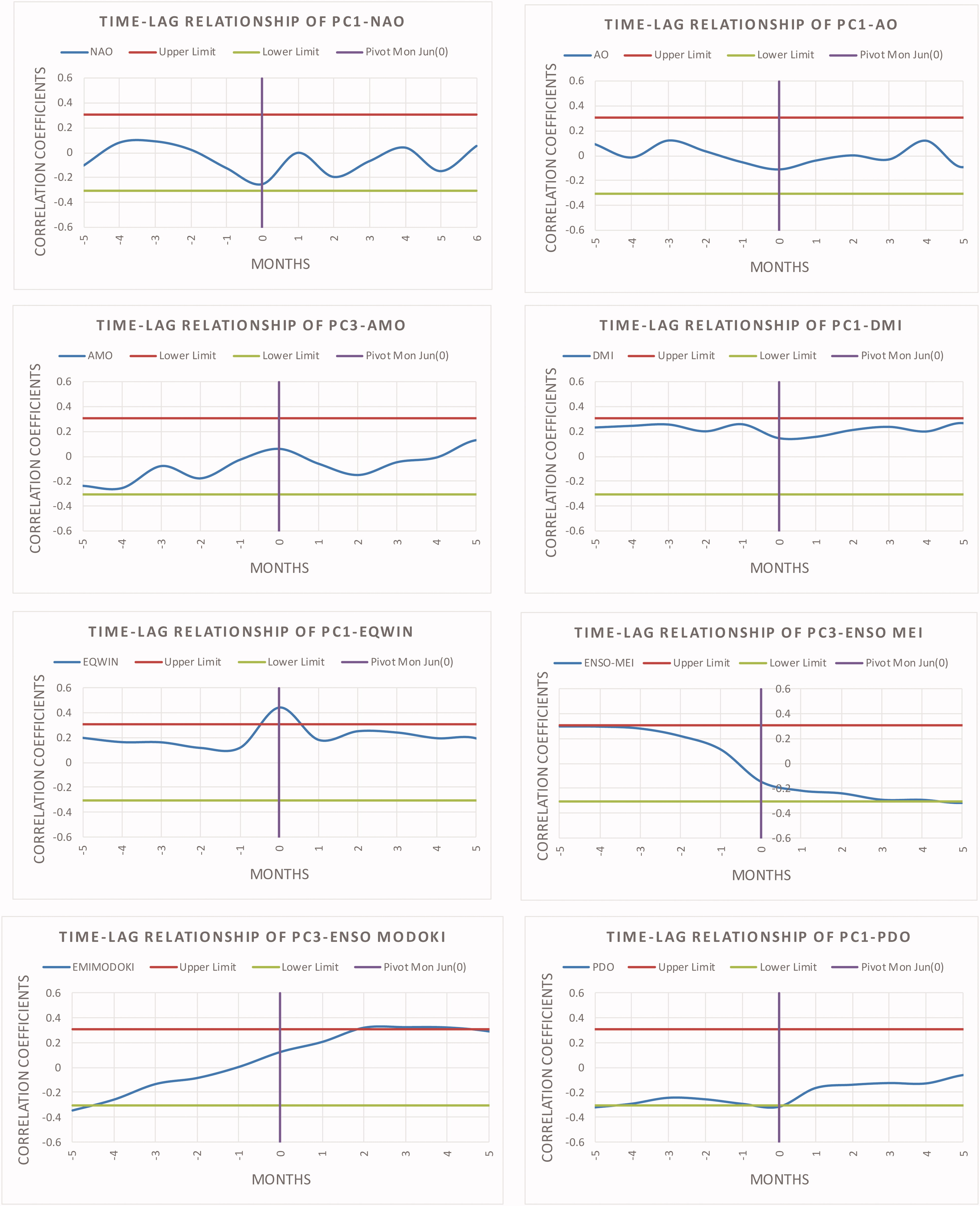
Fig. 25.
Time-lag correlation coefficient between most significant PCs and Climate Indices. June is considered as the pivot month with a value “0” represented by a vertical line whereas negative/positive values along x-axis (Months) indicates preceding/following months from June. Upper and lower limit represents the significance level of 5%.
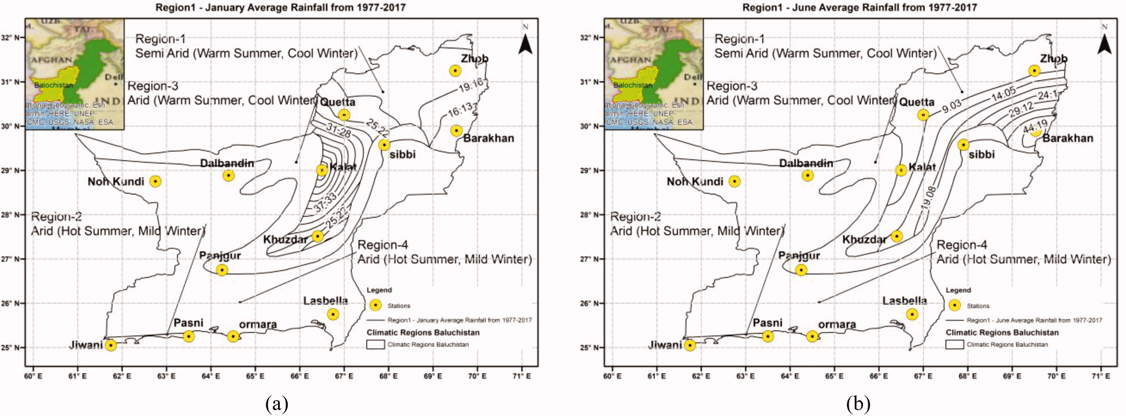
Fig. C1.
(a) Spatial distribution – average Region1 precipitation January. (b) Spatial distribution – average Region1 precipitation June.
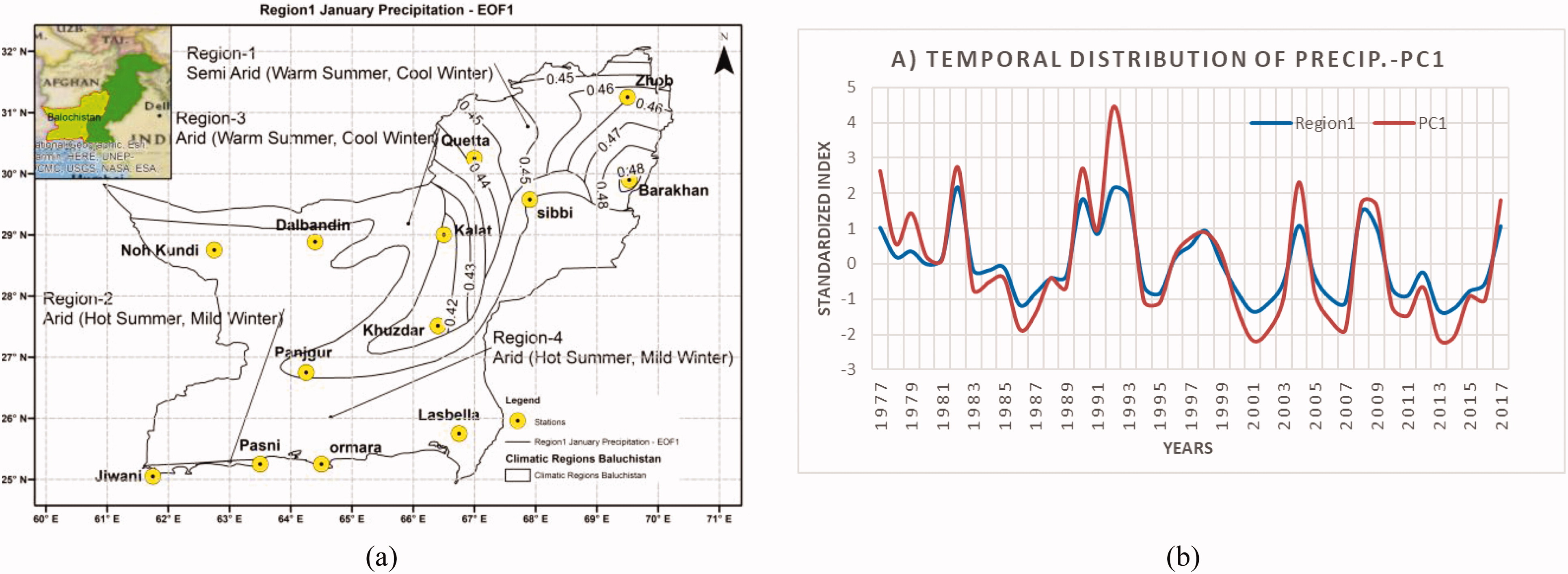
Fig. C2.
(a) Spatial dsistribution of EOF1 of January. (b) Temporal variation of PC-1 of January.
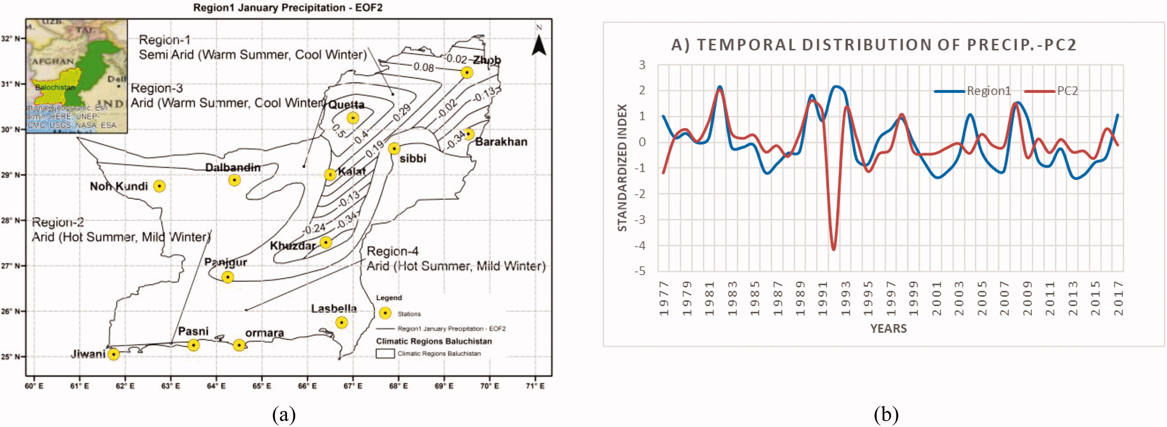
Fig. C3.
(a) Spatial distribution of EOF-2 of January. (b) Temporal variation of PC-2 of January.
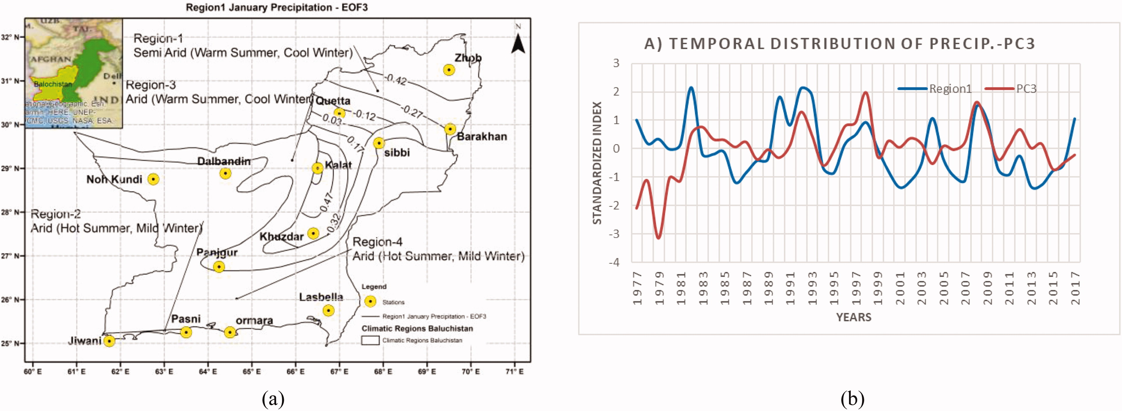
Fig. C4.
(a) Spatial distribution of EOF-3 of January. (b) Temporal variation of PC-3 of January.
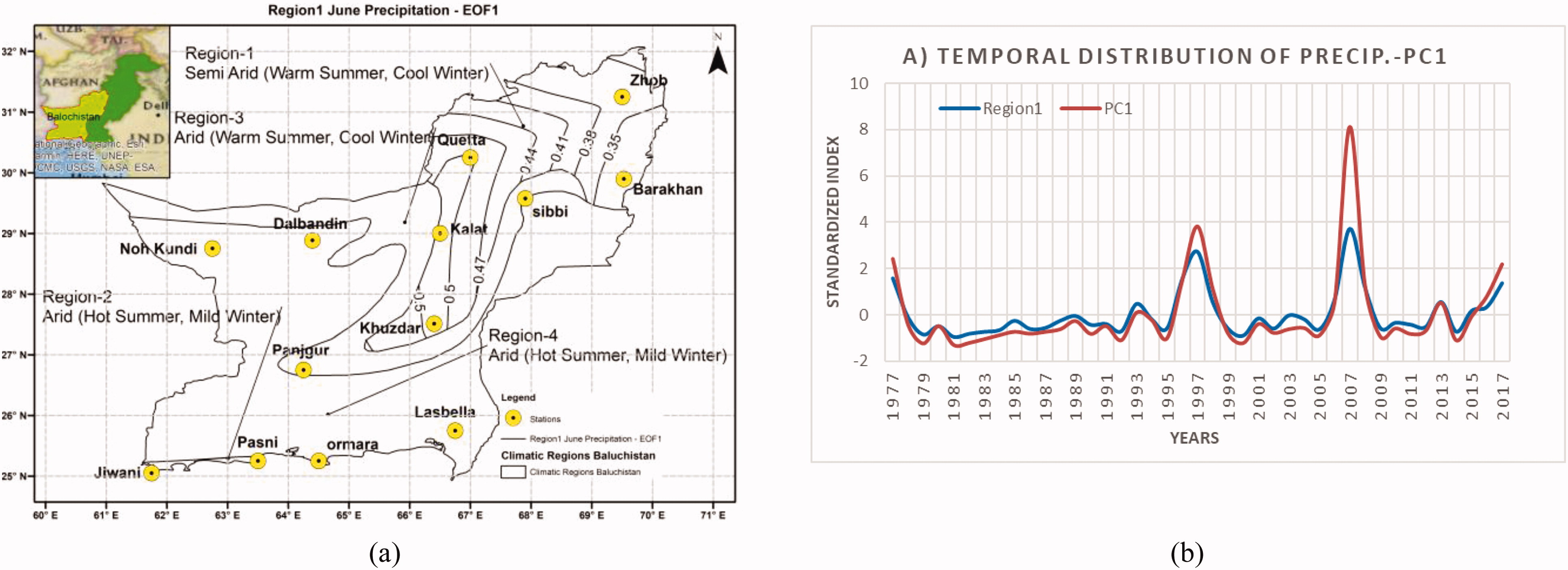
Fig. C5.
(a) Spatial distribution of EOF-1 of June. (b) Temporal variation of PC-1 of June.
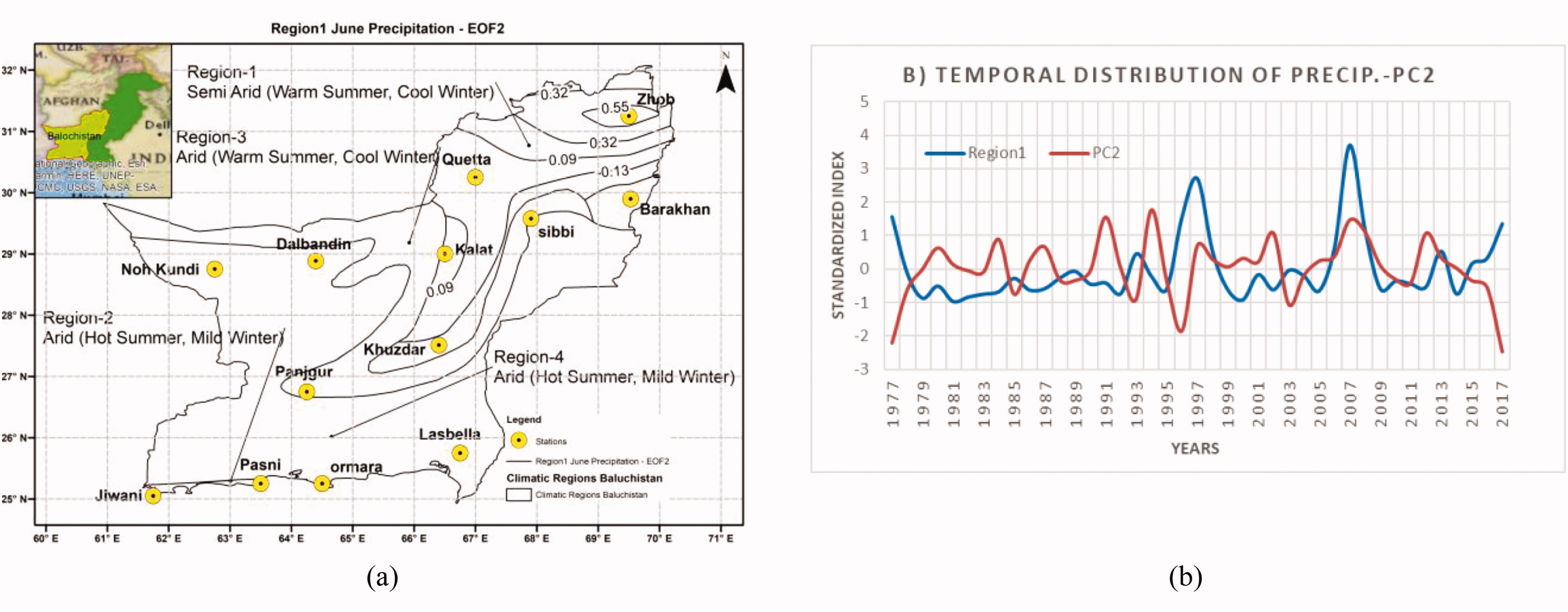
Fig. C6.
(a) Spatial distribution of EOF-2 of June. (b) Temporal variation of PC-2 of June.
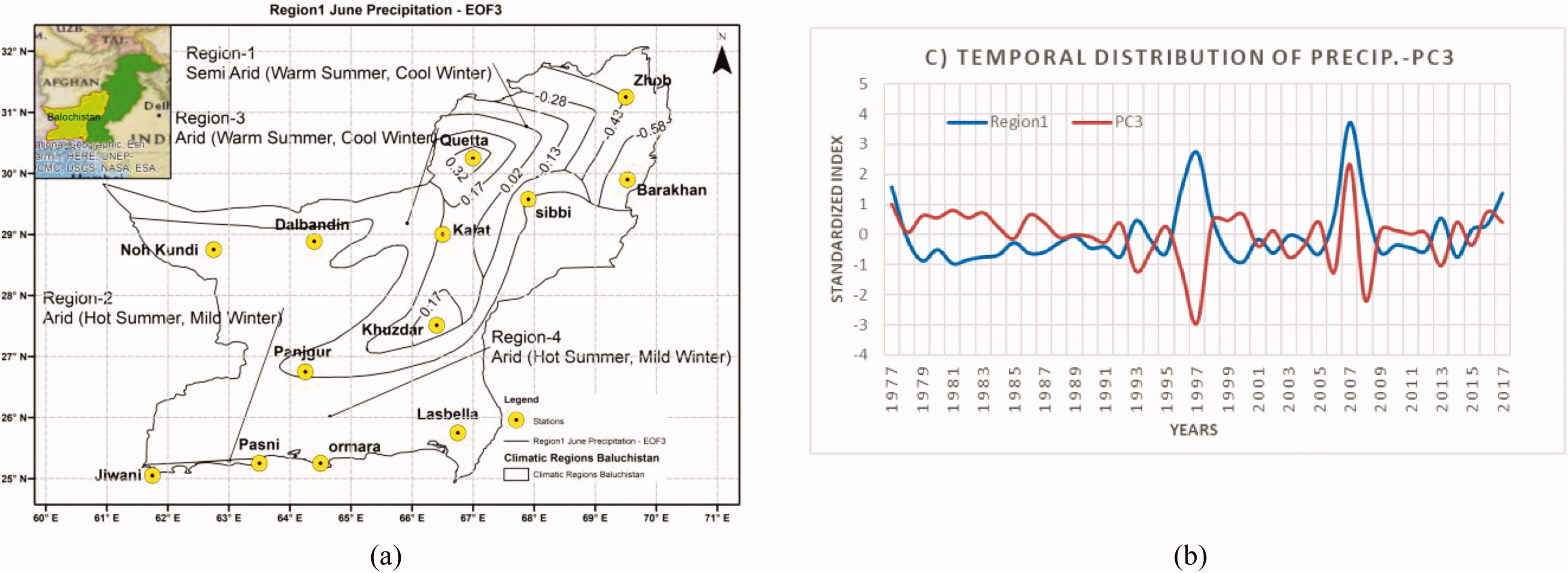
Fig. C7.
(a) Spatial distribution of EOF-3 of June. (b) Temporal variation of PC-3 of June. Refer to Fig. C2b the precipitation index is −0.18 in the year 1983. The EMI-Modoki and NAO index are unusually at −2.98 and +4.824 respectively in January 1983 which may be attributed to the post volcanic eruption of Mount El Chichon-Mexico in March 1982. Similarly, refer to Fig. C5b, the negative precipitation anomaly as is observed in the year June 1982 and June 1991 following the volcanic eruption of Mount El Chichon-Mexico in March 1982 and Mount Pinatubo-Phillipines in June 1991 may be because of variation in climate patterns unfavorable to precipitation due to post volcanic eruption changes in EMI-Modoki and EQWIN indices (Dogar et al., 2017; Dogar, 2018; Dogar and Sato, 2019).
Table 14.
Summary of analysis results for Region1 precipitation and climate indices for June.
PC1 and climate indicesEOF analysisCorrelation b/w PCs and anomalies ofSSTatmospheric circulationZonal winds and OLRNAOWeakSignificant at 11.05%WeakWeakModerate–AOWeakInsignificantWeak–––AMOWeakInsignificantmoderateModerate––DMIWeakInsignificantWeakWeakWeak–EQWINStrongSignificant at 0.4 %StrongModerate–Moderate to StrongENSO-MEIWeakInsignificantStrongWeak––EMI-MODOKIStrongInsignificantWeakWeakWeak–PDOWeakSignificant at 4.57 %StrongStrong––
Table A2.
Influence of NAO on precipitation trends.
Table A3.
Influence of AO on precipitation trends.
Table A4.
Influence of AMO on precipitation trends.
Table A5.
Influence of IOD-DMI on precipitation trends.
Table A6.
Influence of IOD-EQWIN on precipitation trends.
Table A7.
Influence of ENSO-MEI on precipitation trends.
Table A8.
Influence of MODOKI on precipitation trends.
Table A9.
Influence of PDO on precipitation trends.