
Table 1.
The filter matrices and vectors for the Optimal Kalman filter (OKF), reduced-state Kalman filter (RKF) and Schmidt Kalman filter (SKF). The equations for the three filters are obtained through substituting these terms into (3.1) - (3.4). As discussed in section 3.4, we note that while the SKF uses in the innovation only, the complete observation operator is used in the calculation of and
Table 2.
Matrices and vectors used in the true error calculations for Case 1 and 2 described in sections 4.1 and 4.2. The tildes indicate true error covariances. Case 1 corresponds to analysing all scales and includes the OKF. Case 2 corresponds to analysing the large scales only and includes the RKF and SKF. The true analysis error equation, analysis error covariance and forecast error covariance for each case are obtained by substituting the corresponding components into equations (4.1), (4.2) and (4.3) respectively.
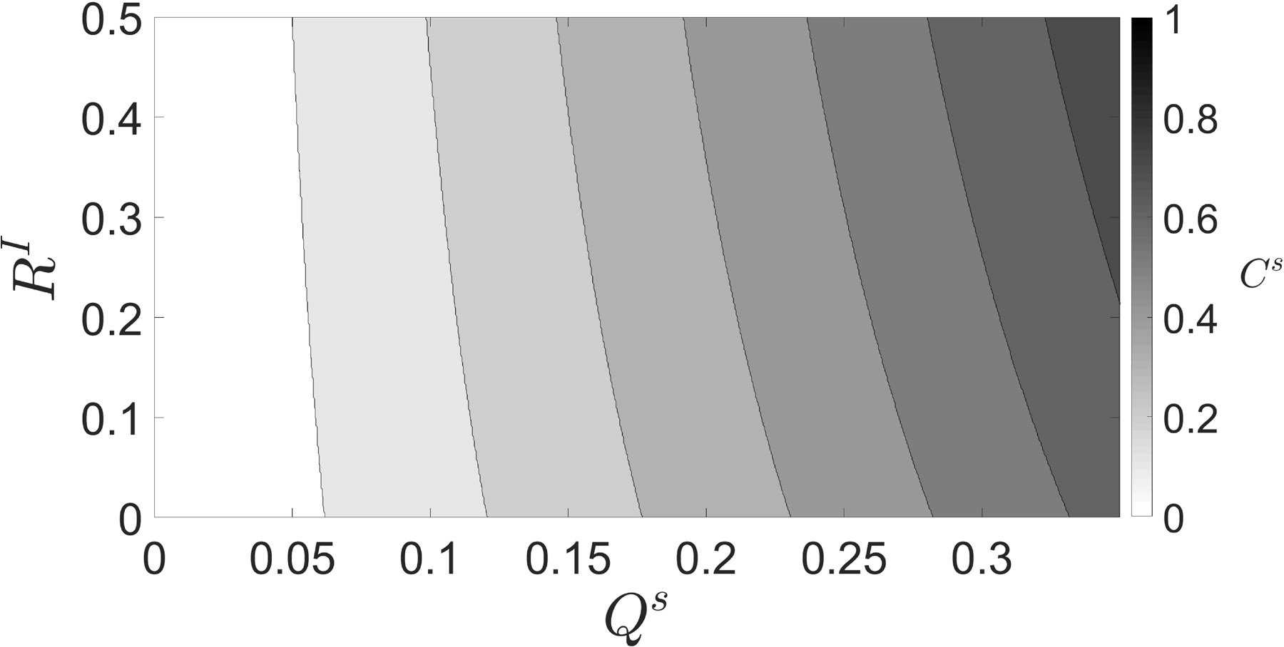
Fig. 1.
Contour plot of the values of that give the minimum true large-scale analysis error variance at the final assimilated observation for the SKF for different ratios of and
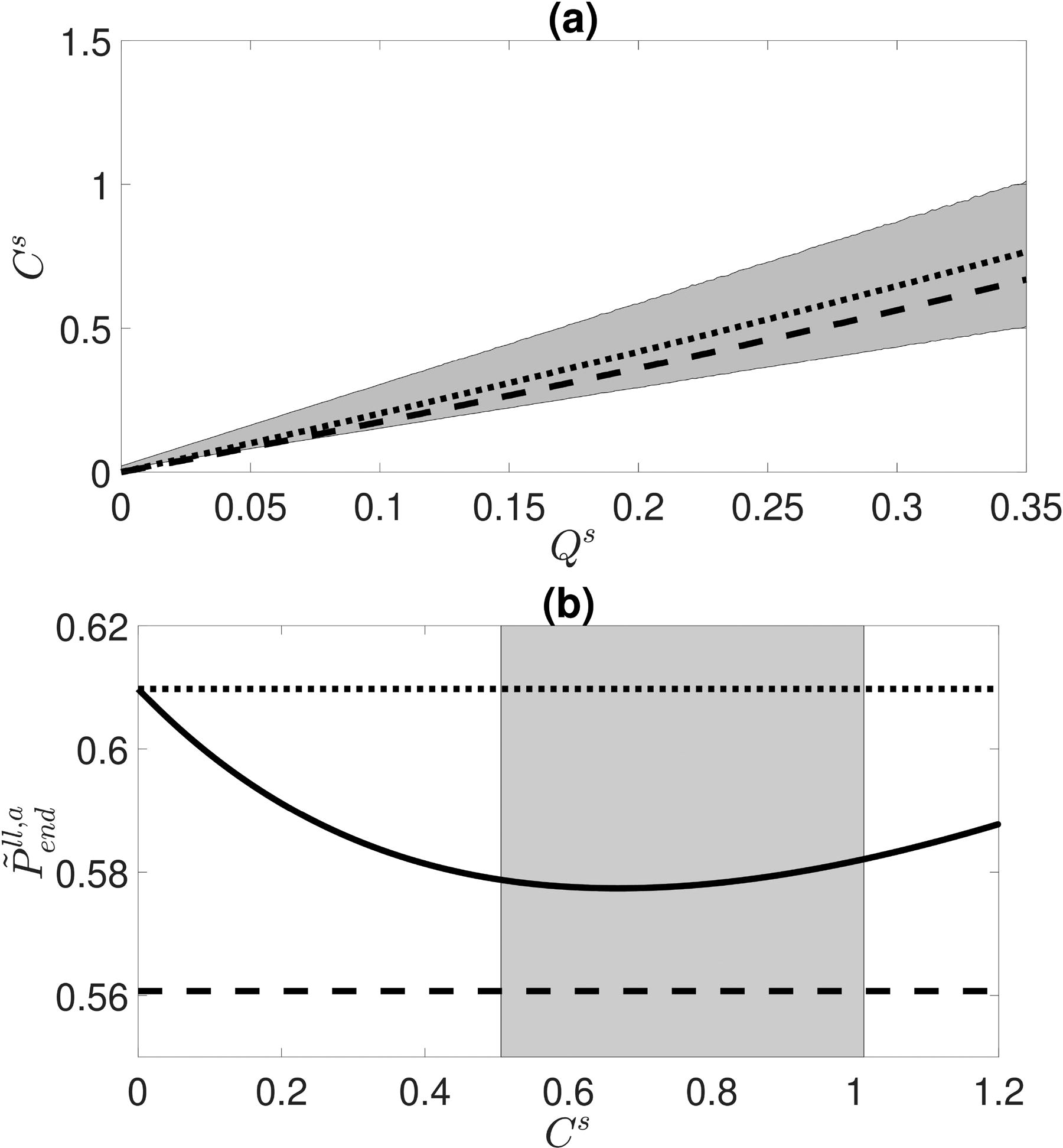
Fig. 2.
(a): The optimal values when (dashed line) and (dotted line) as functions of The grey region shows all points between S (lower edge) and 2S (upper edge) for different values of (b): The effect of changing on the final true large-scale analysis error covariance for the SKF (solid line) when and Also shown are the OKF and RKF true large-scale analysis error variance (lower dashed line and upper dotted line respectively). The grey region shows all points between (left edge) and (right edge). The optimal value of (i.e. the minimum of the solid line) lies in this region.
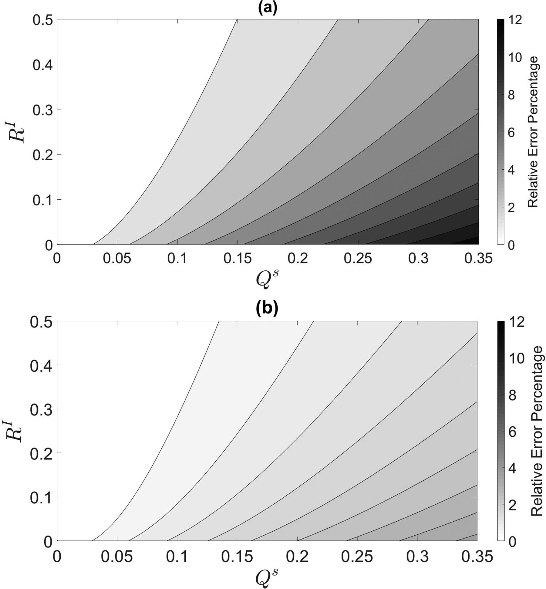
Fig. 3.
(a): Comparison of the RKF to the OKF in terms of relative error percentage given by equation (6.1). (b): Comparison of the SKF with optimal to the OKF at the final time-step in terms of relative error percentage.
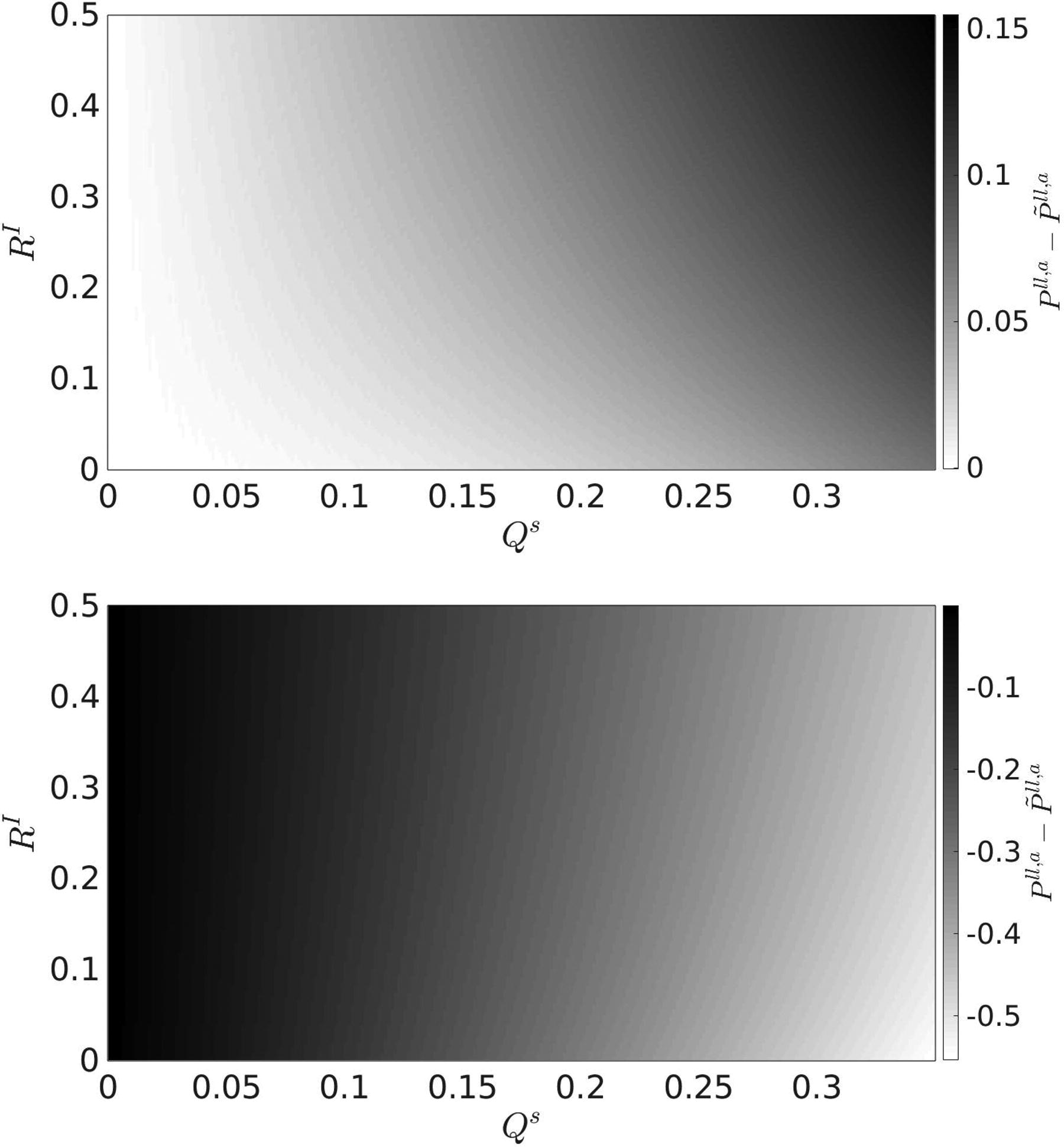
Fig. 4.
(a): Difference between the perceived and true analysis error variances at the final time-step for the SKF with optimal (b): Difference between the perceived and true analysis error variances at the final time-step for the RKF.
Table 3.
RKFbcSKFbcState: x State error covariance: PObservation operator: HObservation error covariance: RInnovation: Innovation covariance: DKalman gain: KForecast model: MModel error covariance: Q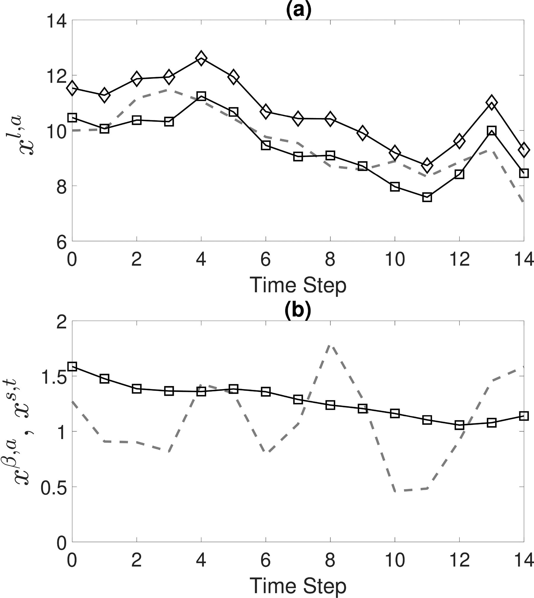
Fig. 5.
(a): The large-scale analysis for the SKFbc (square markers) and SKF (diamond markers) obtained through assimilation of biased observations to recreate the true large-scale state (grey dashed line). For this realization the large-scale analysis mean-square-error for the SKFbc is 0.29 and for the SKF is 1.53. (b): The SKFbc bias analysis estimate (square markers) and the true small-scale state (grey dashed line) for the same realization as panel (a).
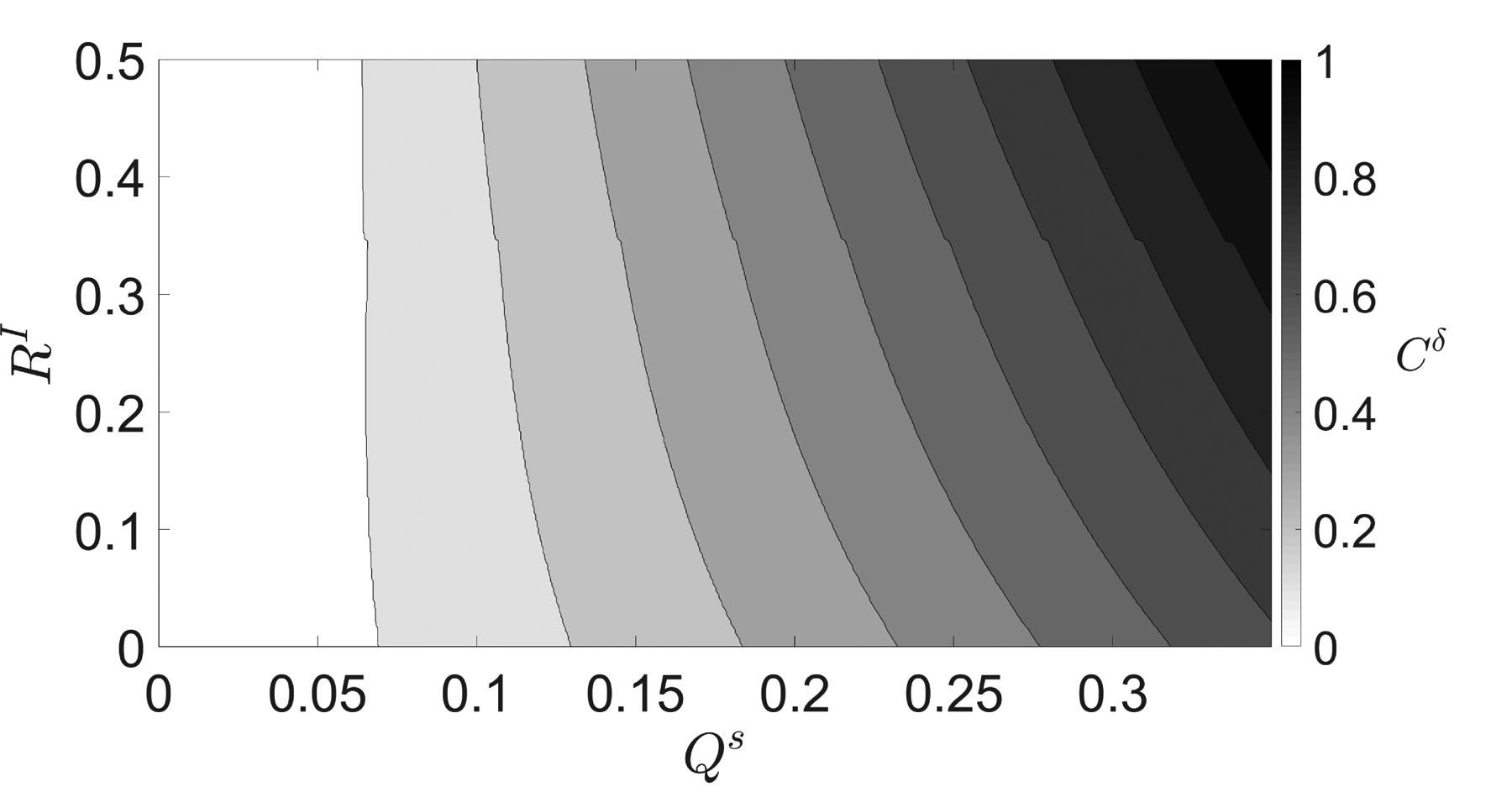
Fig. 6.
The values of which give the minimum true large-scale analysis error variance at the end of the assimilation window for the SKFbc.
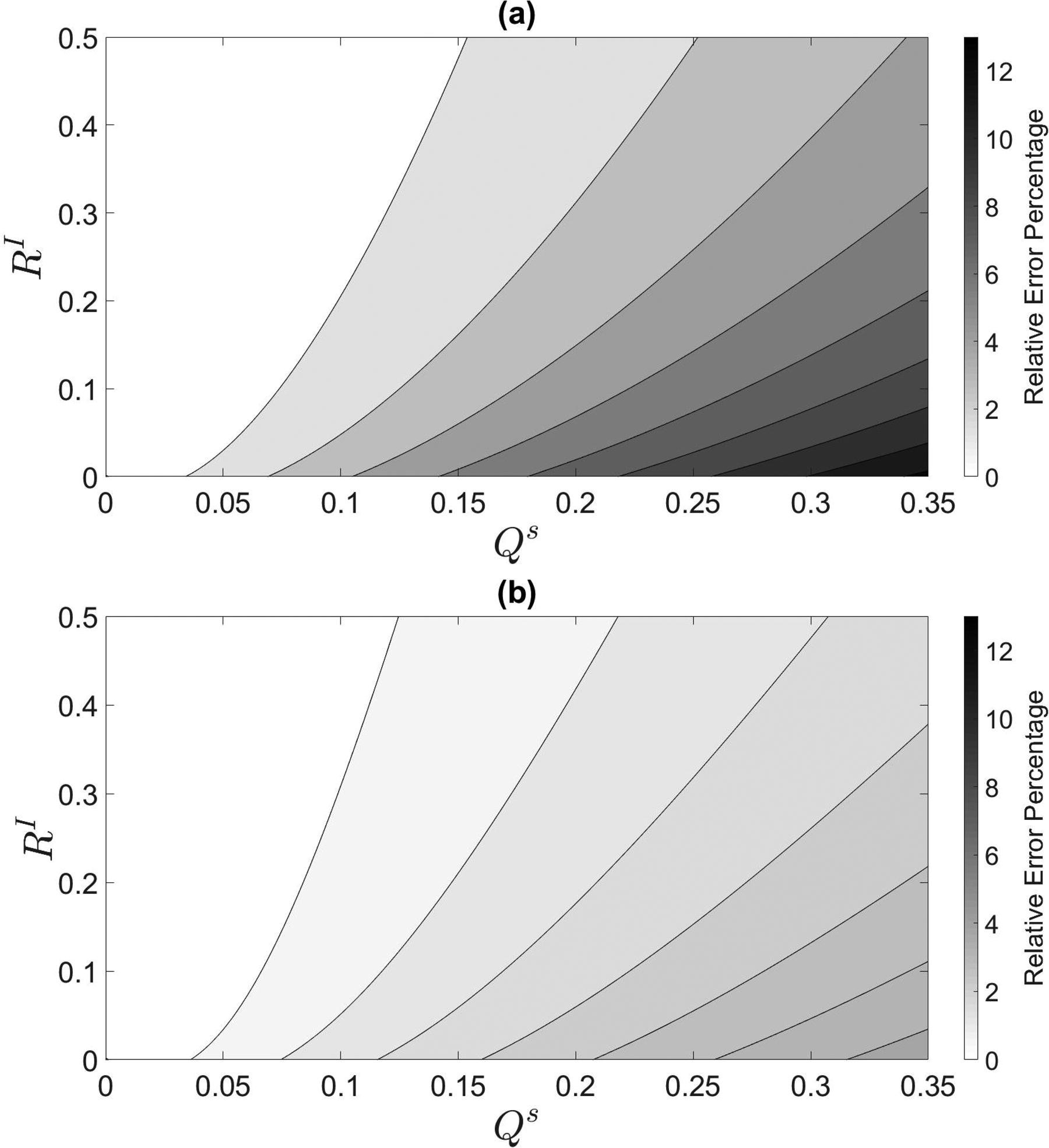
Fig. 7.
(a): Comparison of the RKFbc to the OKF in terms of relative error percentage given by equation (6.1). (b): Comparison of the SKFbc with optimal to the OKF at the final time-step in terms of relative error percentage.