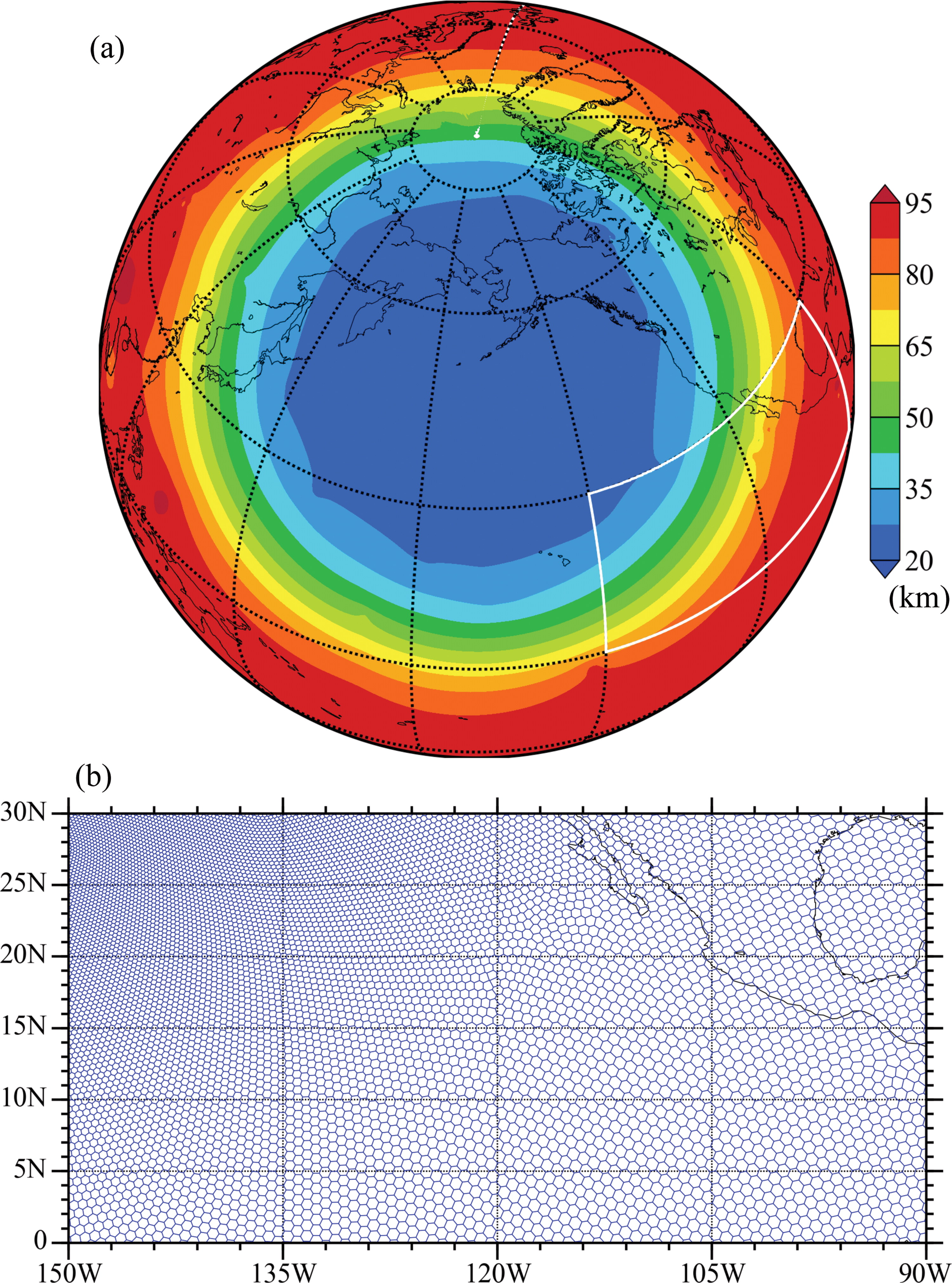
Fig. 1.
(a) Global distribution of distances between neighbouring cells (shaded in colour) of a variable resolution grid with horizontal resolutions ranging from 25 km to 92 km. The centre of refined resolution is at [50° N, 170° W]. (b) Cell distribution of variable resolution grid cells within a zoomed region indicated by the white box in (a). The area in (a) is shown using the equidistant conic projection, and the area in (b) is shown using the equidistant cylindrical projection.
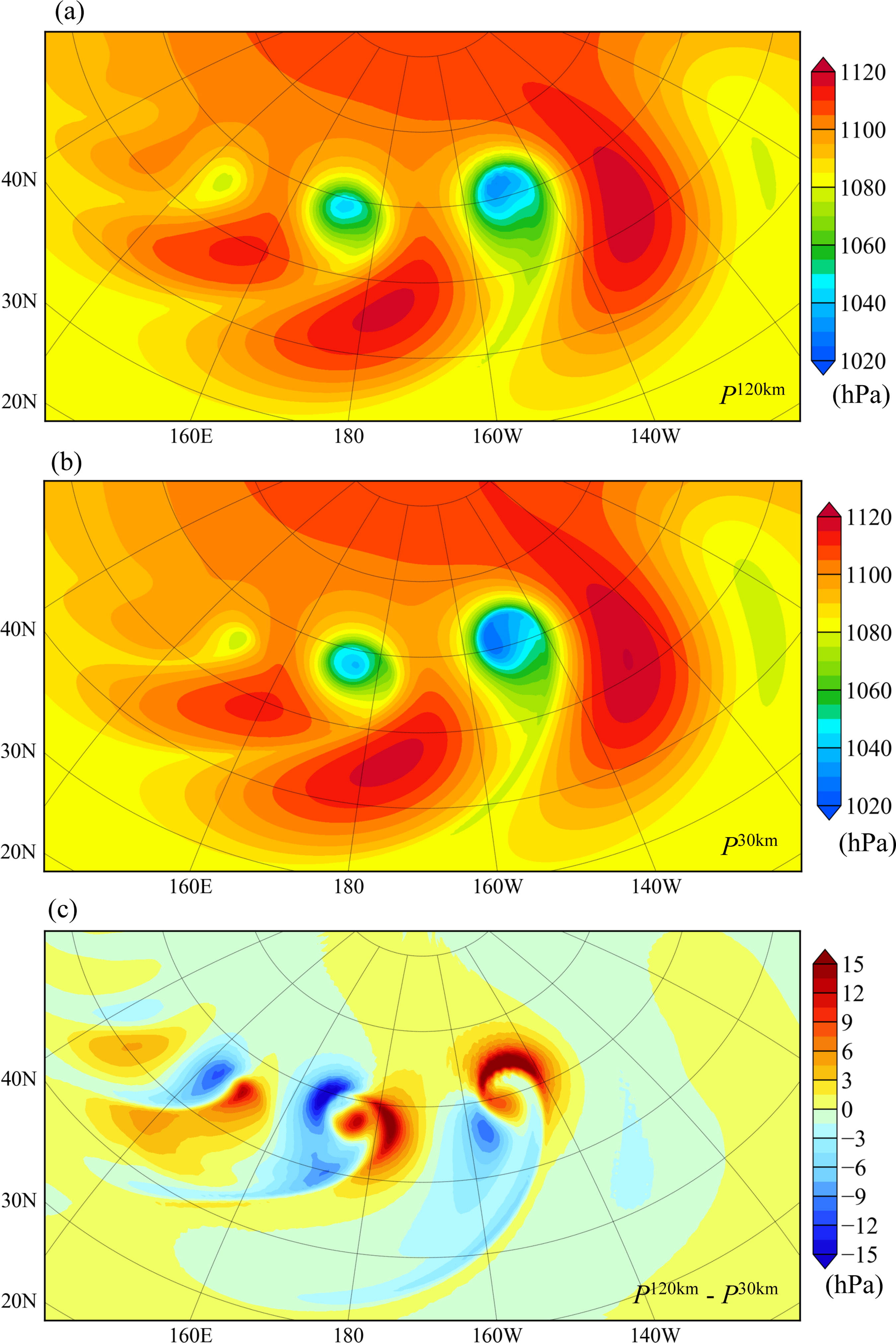
Fig. 2.
Surface pressure distributions (unit: hPa) after nine-day integrations with uniform resolutions of (a) 120 km and (b) 30 km. (c) Differences in surface pressure between the 120 and 30 km resolutions.
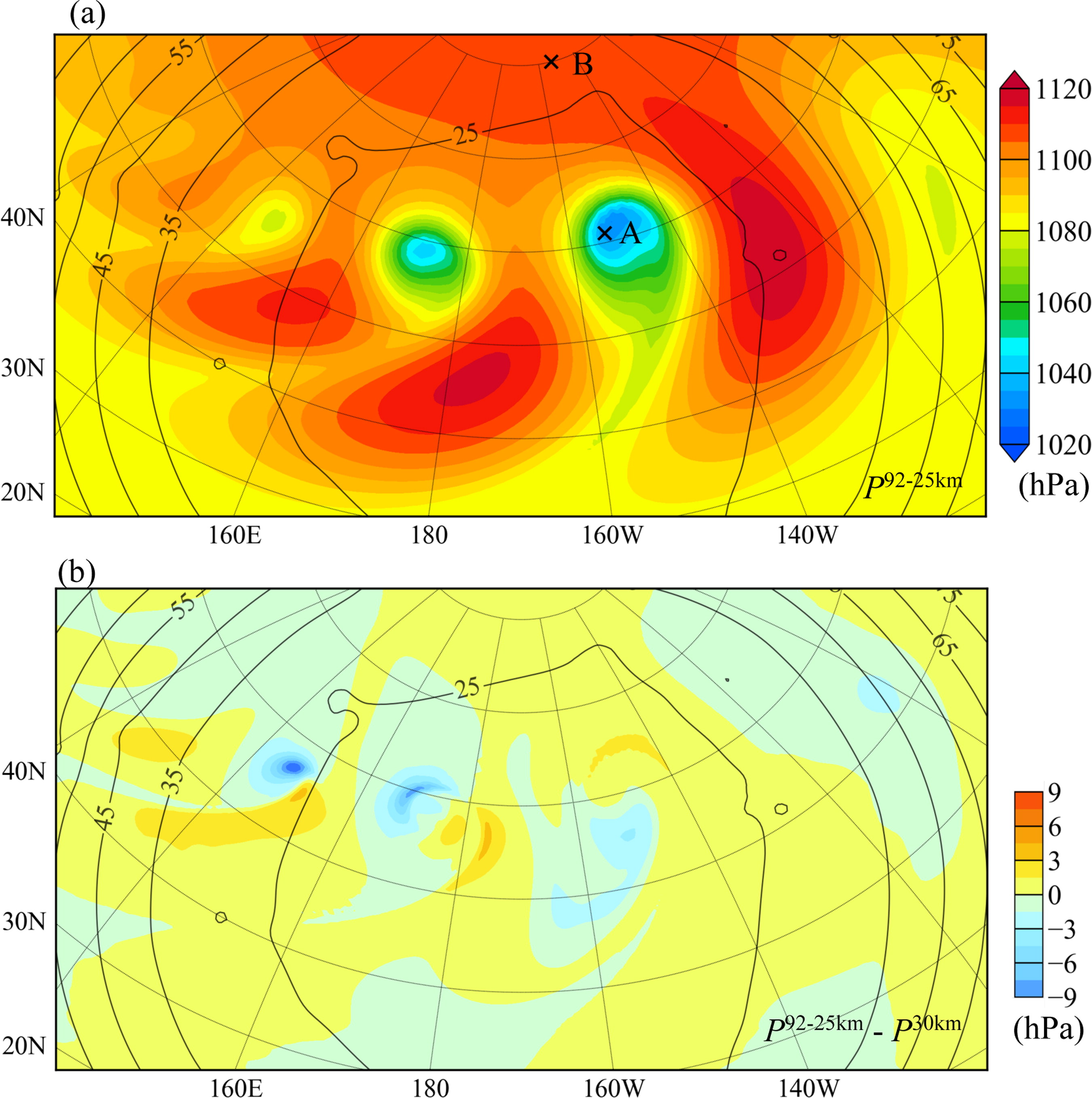
Fig. 3.
(a) Surface pressure distribution (unit: hPa) after a nine-day integration with a variable resolution. (b) Differences in surface pressure between the variable-resolution and 30-km uniform resolutions. Point A is at [61° N, 153° W], and point B is at [80° N, 153° W]. The black contours are the distances (unit: km) between neighbouring cells shown in Fig. 1a.
Table 1.
Computational costs for 24-h integrations of a global MPAS-A non-linear model at 120-km and 30-km quasi-uniform resolutions and a variable resolution varying from 25 km to 92 km, as well as the costs for tangent linear and adjoint models at the variable resolution.
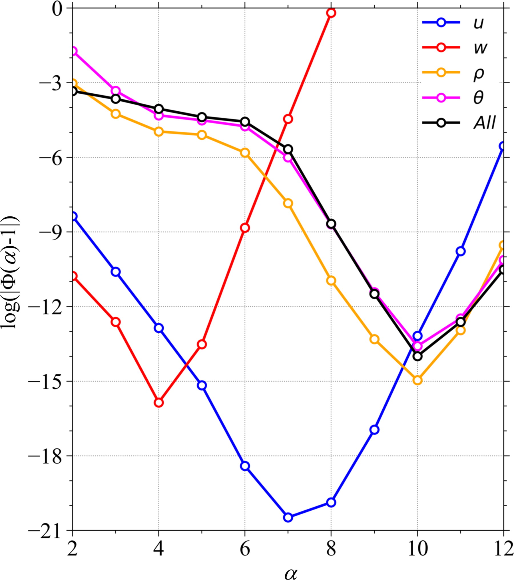
Fig. 4.
Variations in the function |Φ(α) – 1| for the correctness check of the MPAS-A tangent linear model for the 24-h forecast length when the initial conditions for variables u, w, ρ and θ are separately perturbed, where α is the scale factor of initial perturbations.
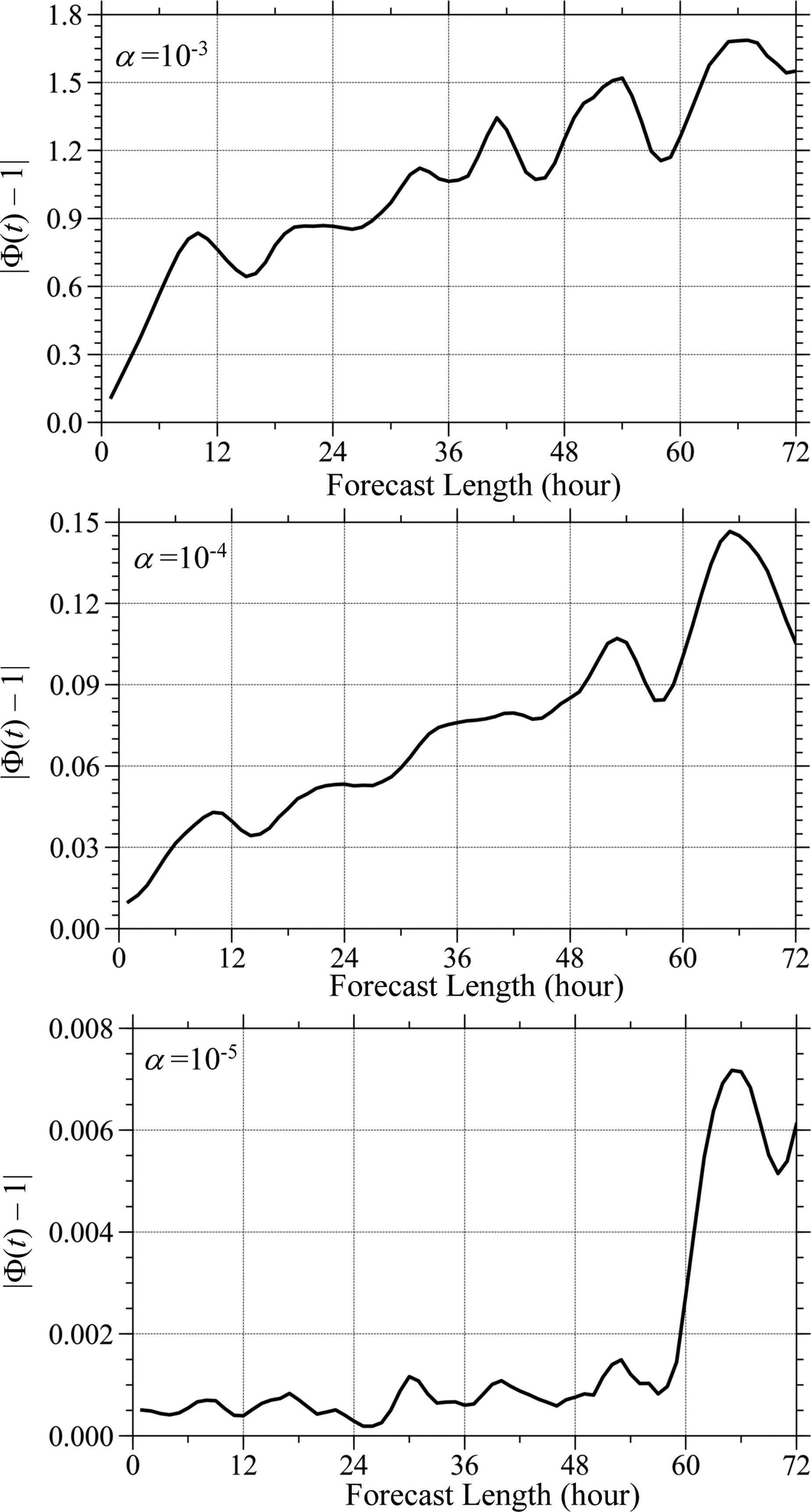
Fig. 5.
Temporal evolutions of the global mean |Φ(t) – 1| with respect to the forecast length when α = 10–3, 10–4 and 10–5.
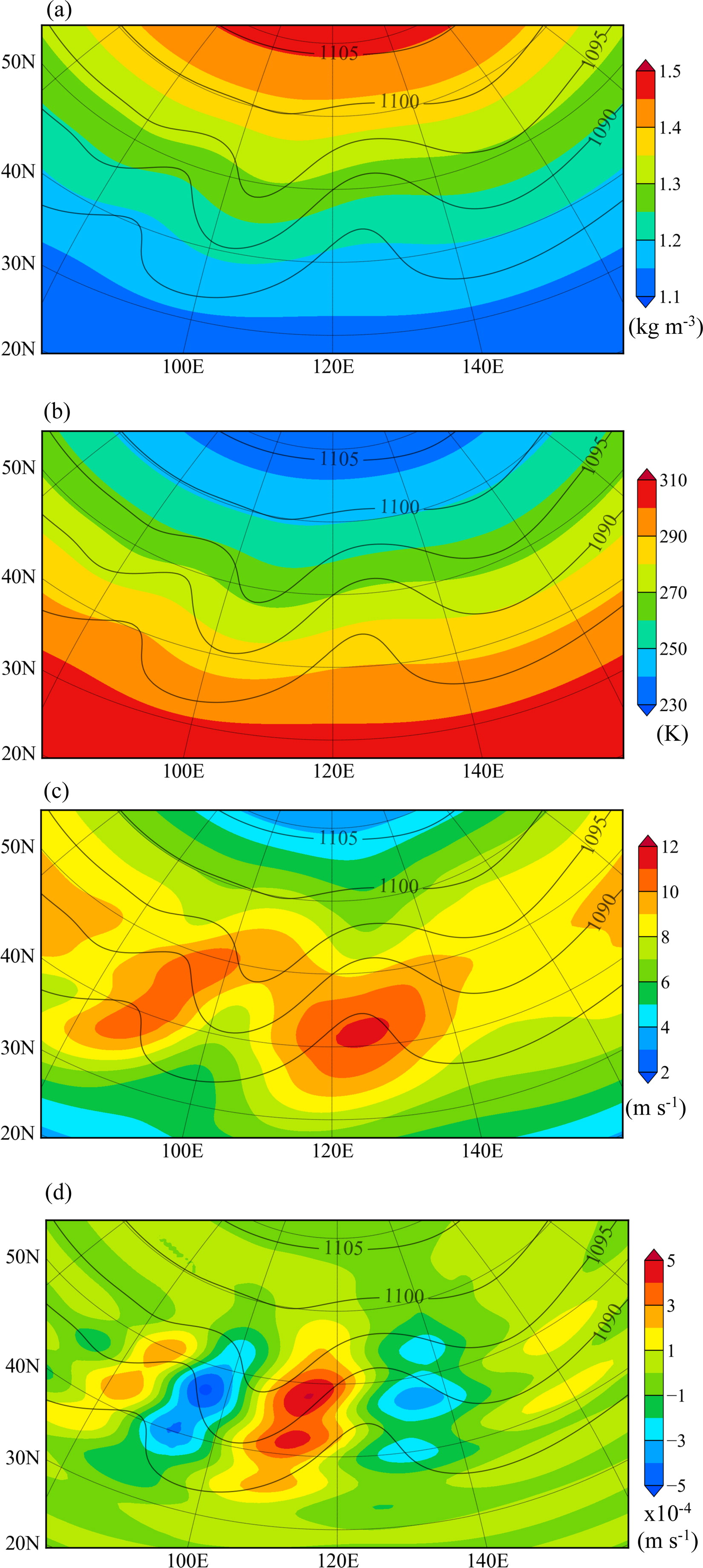
Fig. 6.
(a) ρ, (b) θ, (c) u and (d) w and surface pressure (black contours, unit: hPa) at 0000 UTC of day 5 with the variable resolution mesh.
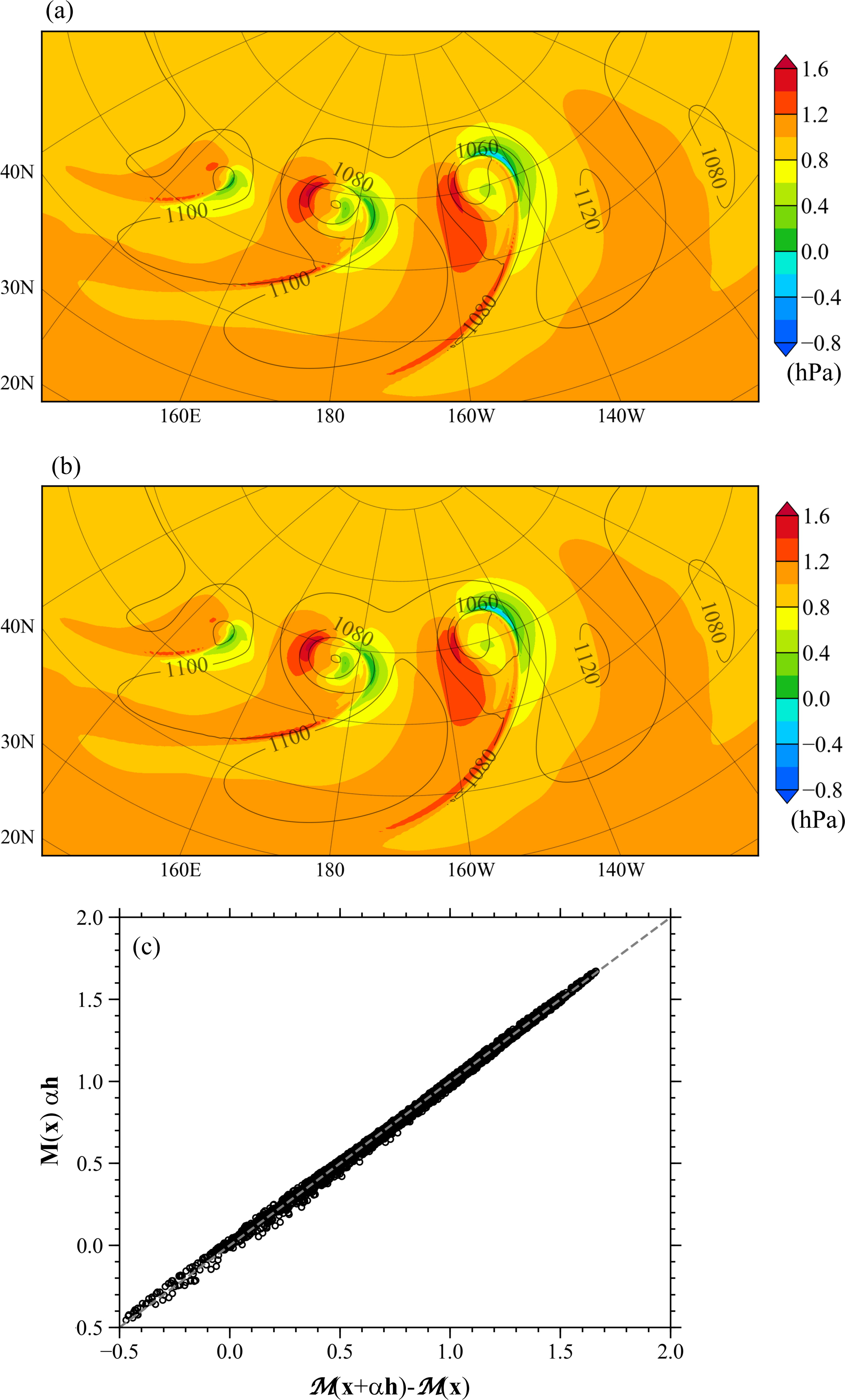
Fig. 7.
(a) Differences in surface pressure (unit: hPa) after four-day integrations of the non-linear forward model with and without perturbations [i.e. (x + αh) – (x)], and (b) the four-day perturbation forecast of the tangent linear model [M(x)αh], where a perturbation of α = 10–3 is given to all state variables (u, w, ρ, θ, and qv) on day 5, as shown in Fig. 6. Surface pressures from the non-linear forward model on day 9 are shown in (a) and (b) as black contours. (c) Scatter plot of M(x)αh as a function of [(x + αh) – (x)]. The linear fit is y = 0.983x + 0.0179, with a root-mean-square error of 0.00454 hPa.
Table 2.
Correctness check results of the newly developed MPAS-A adjoint model when it is integrated for 1, 3, 6, 9 and 12 h.
[i] LHS: left-hand side of Equation (5); RHS: right-hand side of Equation (5).
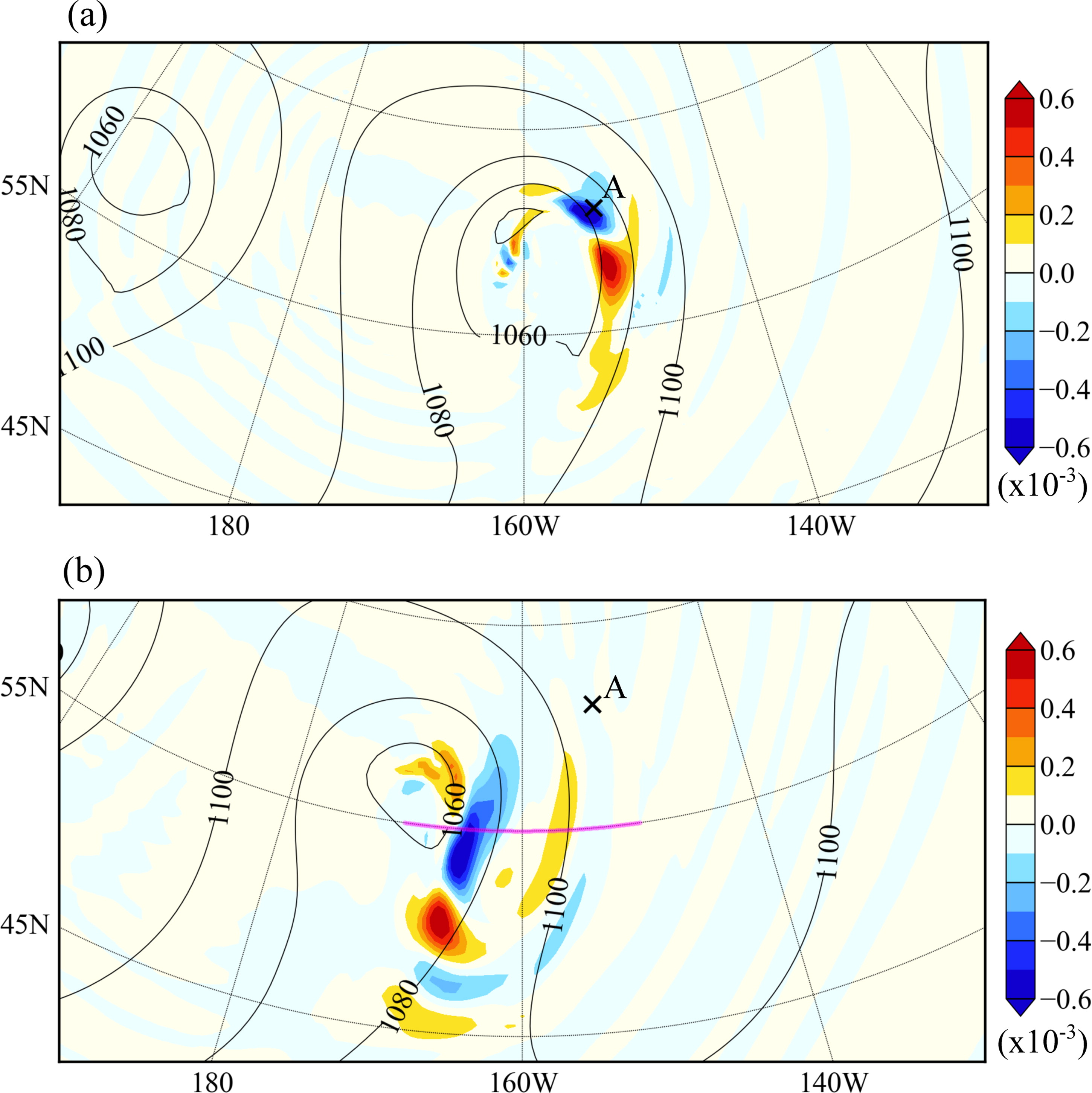
Fig. 8.
Relative sensitivities of the surface pressure at point A at 0000 UTC of day 9 (see Fig. 3a) to the ρ field at the surface level at (a) 1200 UTC and (b) 0000 UTC of day 8 (shaded in colour, ×10–3). Black contours show the surface pressures at 1200 UTC and 0000 UTC of day 8 in (a) and (b), respectively.
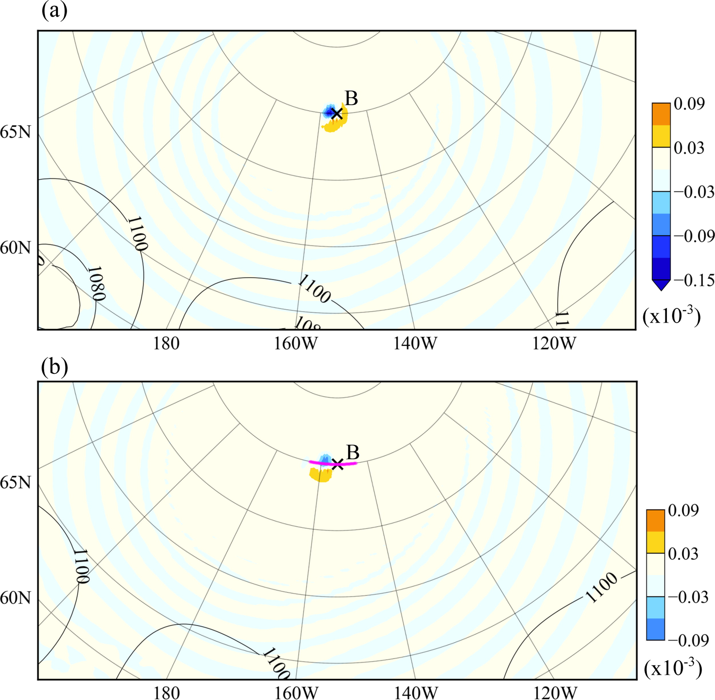
Fig. 9.
Relative sensitivities of the surface pressure at point B at 0000 UTC of day 9 (see Fig. 3a) to the ρ field at the surface level at (a) 1200 UTC and (b) 0000 UTC of day 8 (shaded in colour, ×10–3). Black contours show the surface pressures at 1200 UTC and 0000 UTC of day 8 in (a) and (b), respectively.
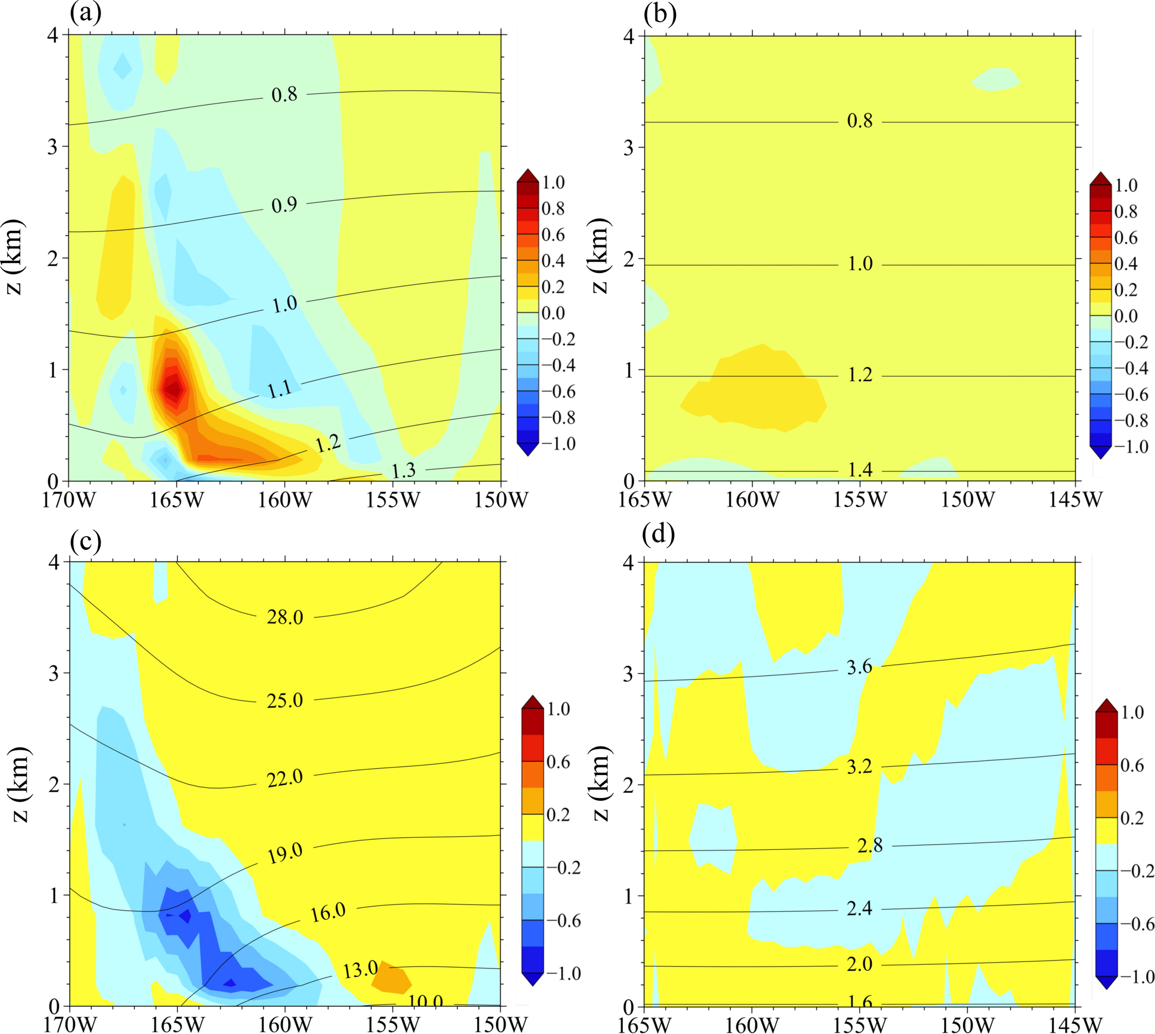
Fig. 10.
Cross-sections of relative sensitivities of the surface pressure at point A (left panels) and point B (right panels) at 0000 UTC of day 9 (see Fig. 3a) to (a, b) the ρ field (×10–3) and (c, d) the u field (×10–5) at 0000 UTC of day 8 (shaded in colour). The ρ field at 0000 UTC of day 8 is shown in (a, b) (black curves), and the u field at 0000 UTC of day 8 is shown in (c, d) (black curves).