
Table 1.
Arrangement and parameters of the CWB ensemble system for typhoon.
Global
GlobalT511L607-day20 members ensembleT511L607-daybased ontangent/adjointT42L6048-hoursingular vectorAround TC
East Asia
48-hour
[i] The ensemble prediction system uses the same resolution as the deterministic model in T511L60. They are global spectral models. The tangent/adjoint model in T42L60 is the simplified version of T511L60. The singular vectors are from the dry total energy with two local projection domains. The TC domain is around the TC centre and moves with the TC. The East Asia domain is shown in the table. The optimal finite time of the singular vector is 48-hour.
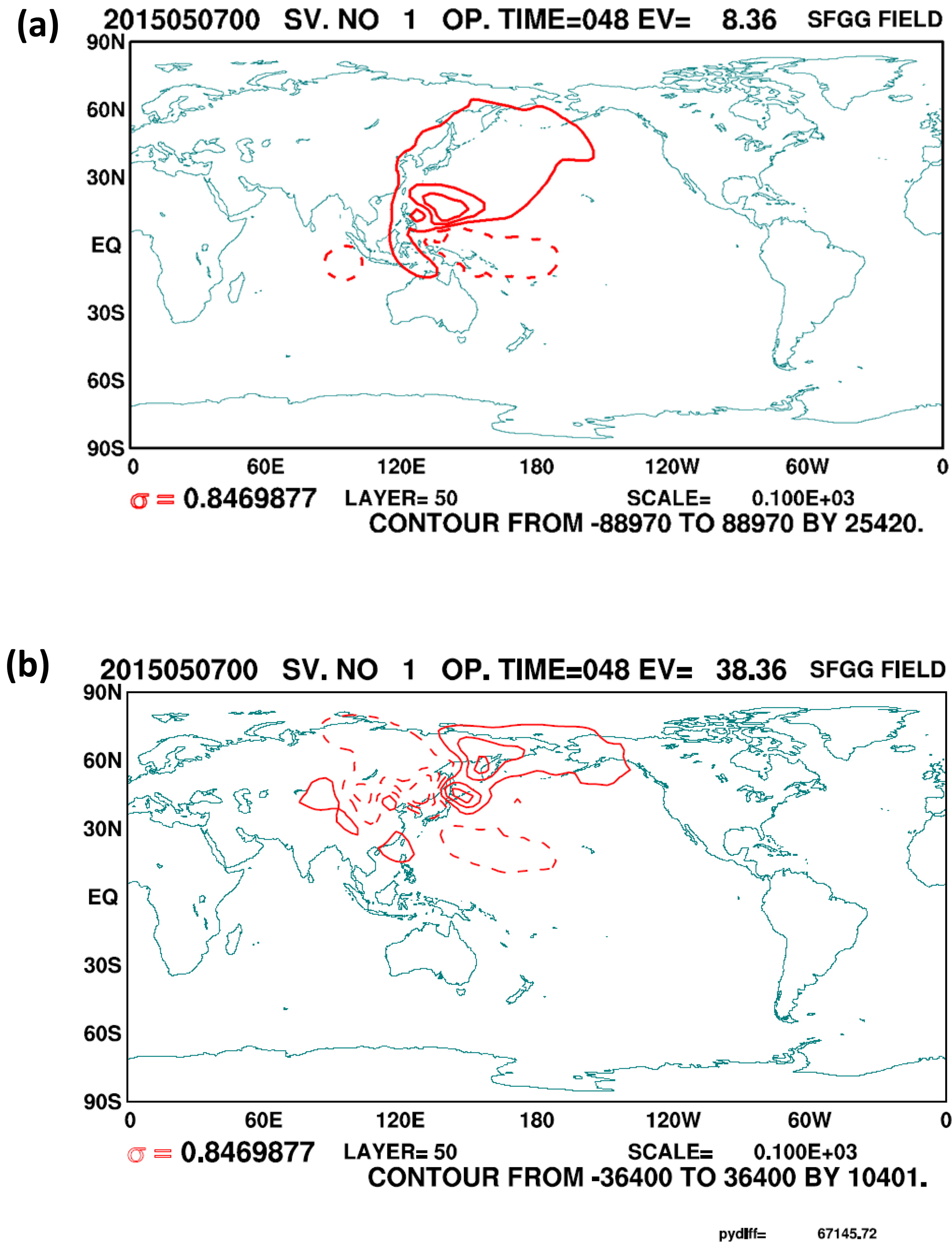
Fig. 1.
Original singular vectors from T42L60 model are shown as stream function (m2/s) based on 0000 UTC 7 May 2015 basic flow. (a) The first one singular vector in the TC domain. (b) The first one singular vector in East Asia domain.
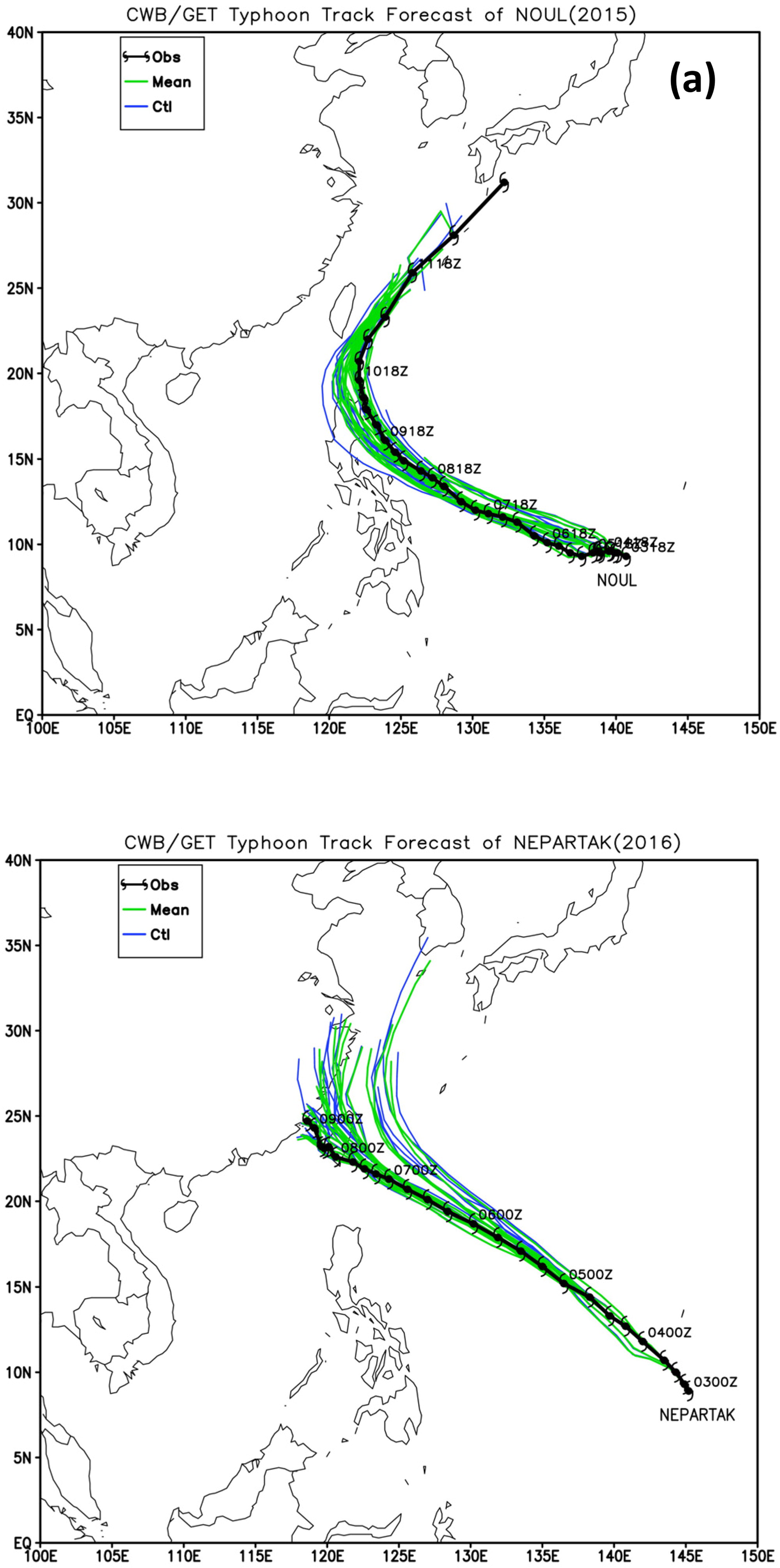
Fig. 2.
Typhoon tracking and forecasting composite maps. The green lines indicate ensemble mean, the blue lines indicate the deterministic run, and the black line indicates the best track. (a) Typhoon Noul. (b) Typhoon Nepartak.
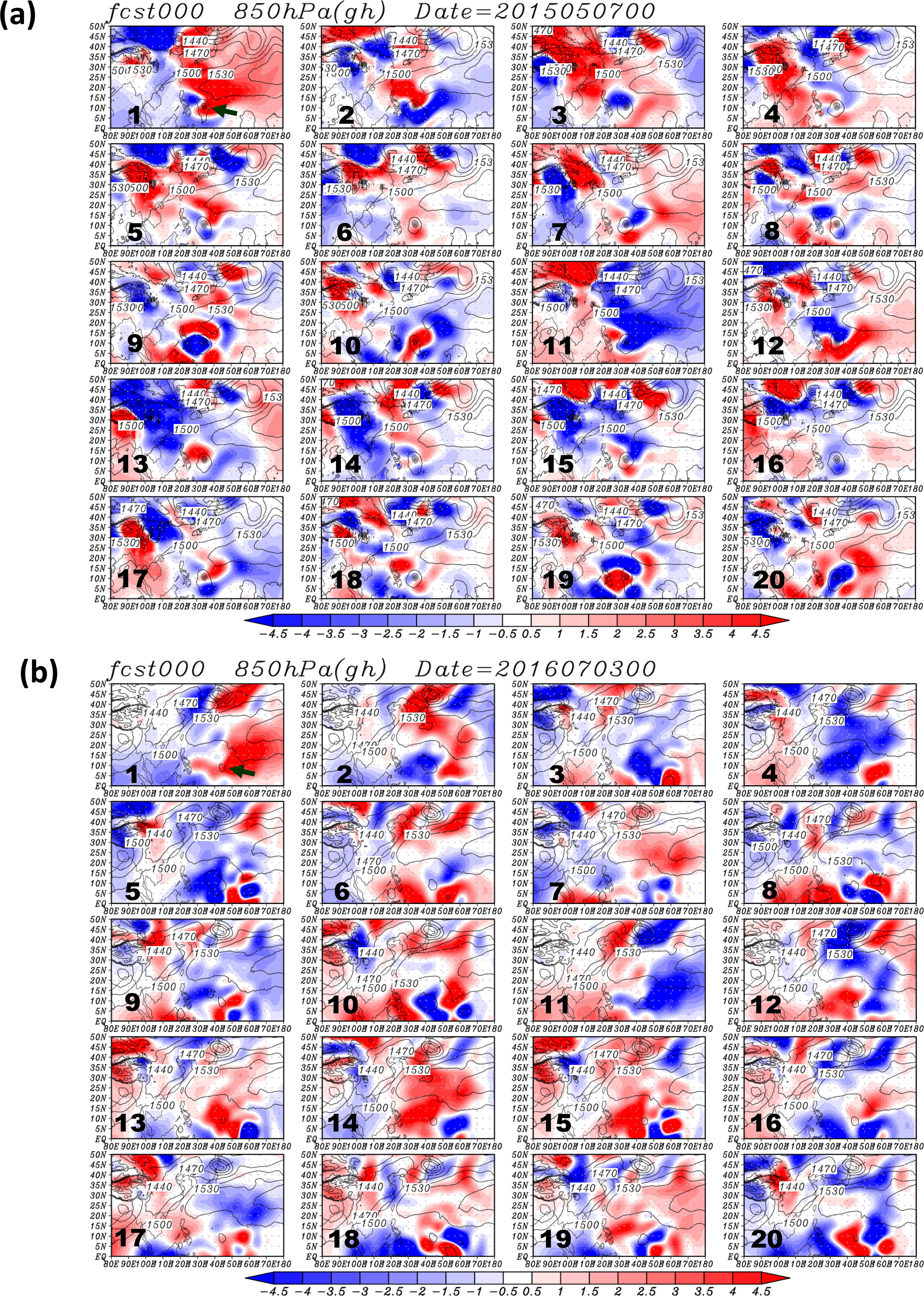
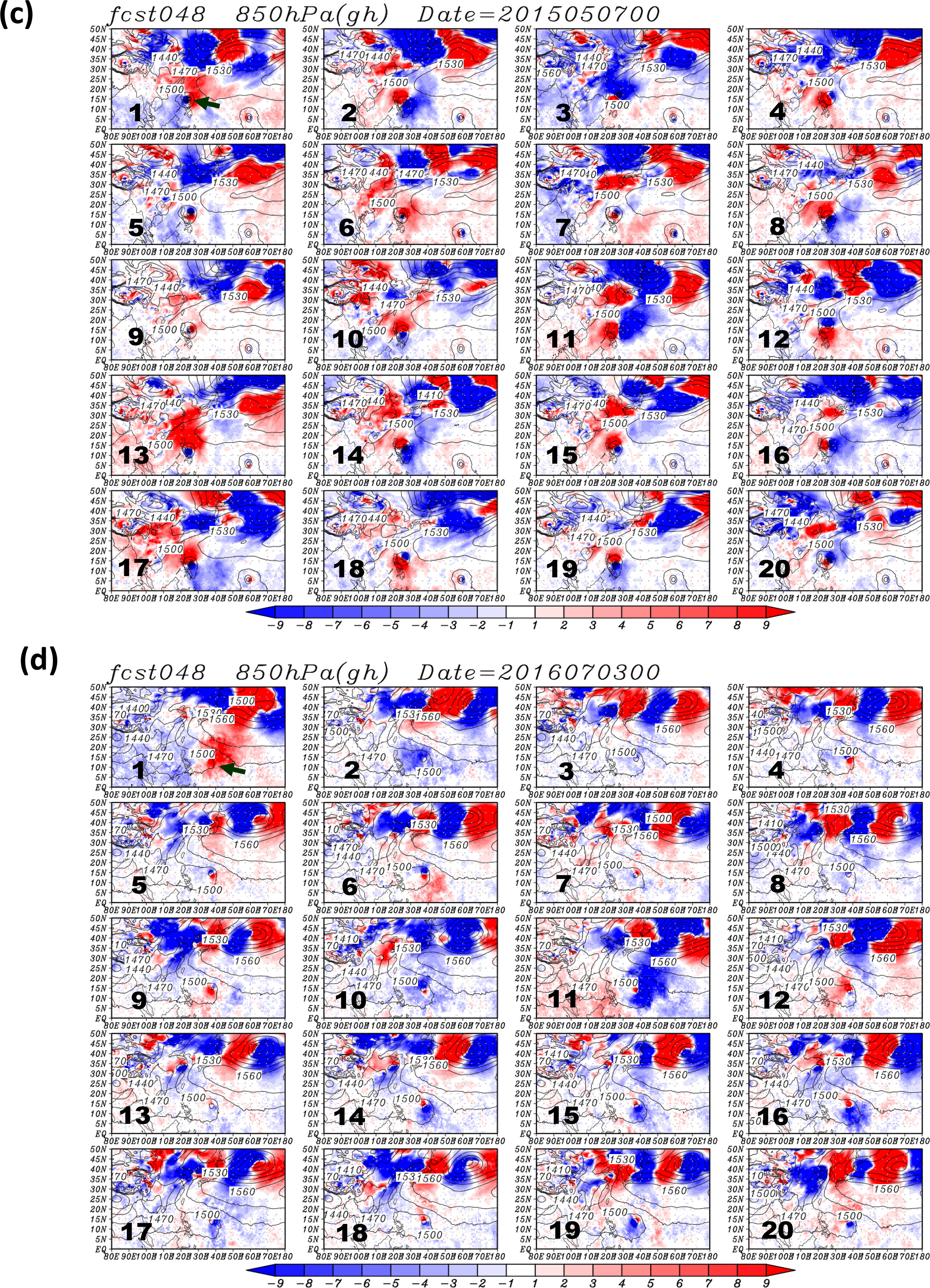

Fig. 4.
Longitudinal-pressure dry total energy (J/kg) cross-sections of 20 members of singular vector perturbations. The longitude range is from to and the vertical range is from 1000 to 100 hPa. (a) At 0000 UTC 7 May 2015, the latitudinal average is taken from to (b) at 0000 UTC 3 July 2016, the latitudinal average is from to The E-vector vertical component is 10 times of original.
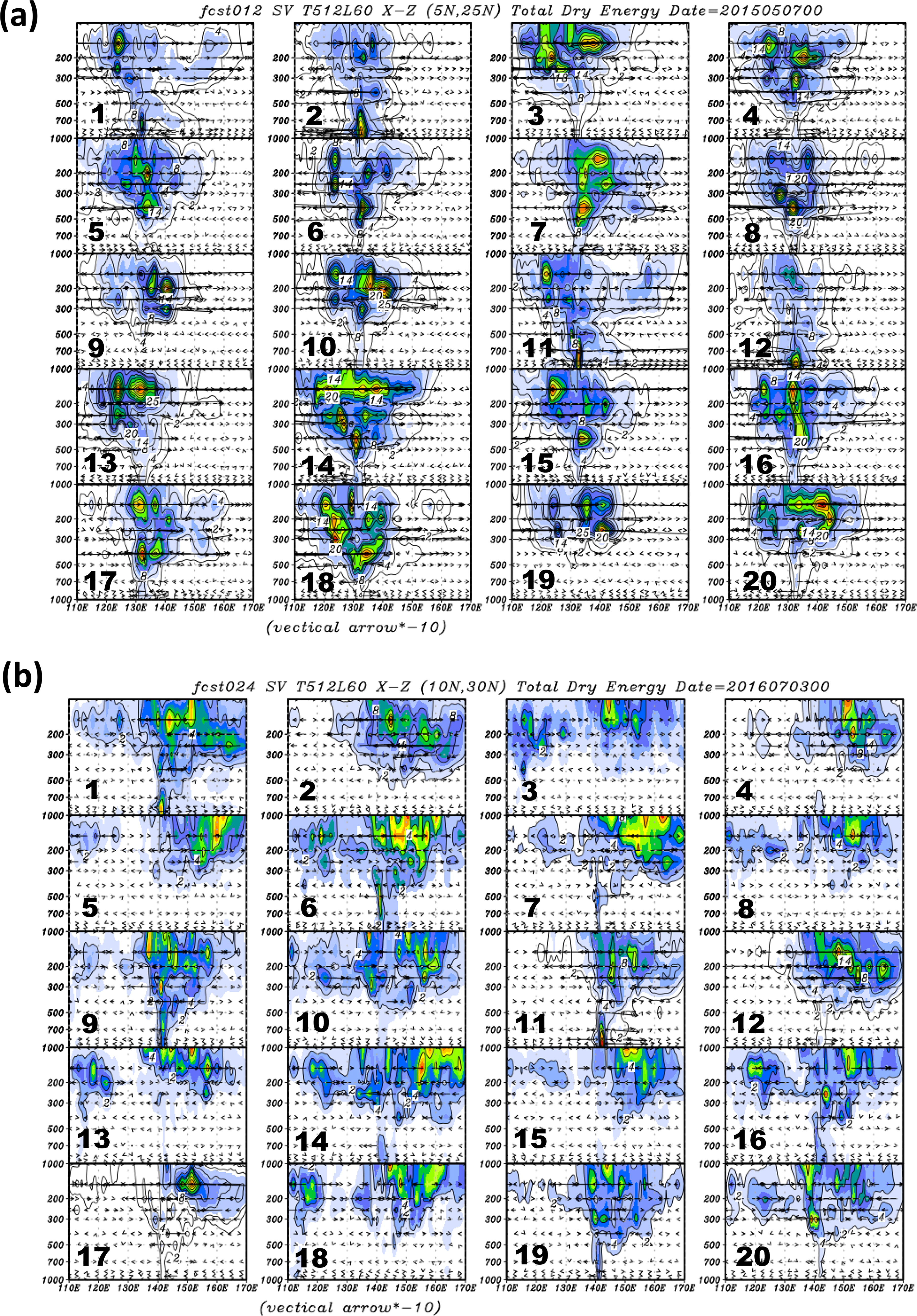
Fig. 5.
As in Fig. 4 (a) For the 12-hour forecast of 0000 UTC 7 May 2015. (b) For the 24-hour forecast of 0000 UTC 3 July 2016.
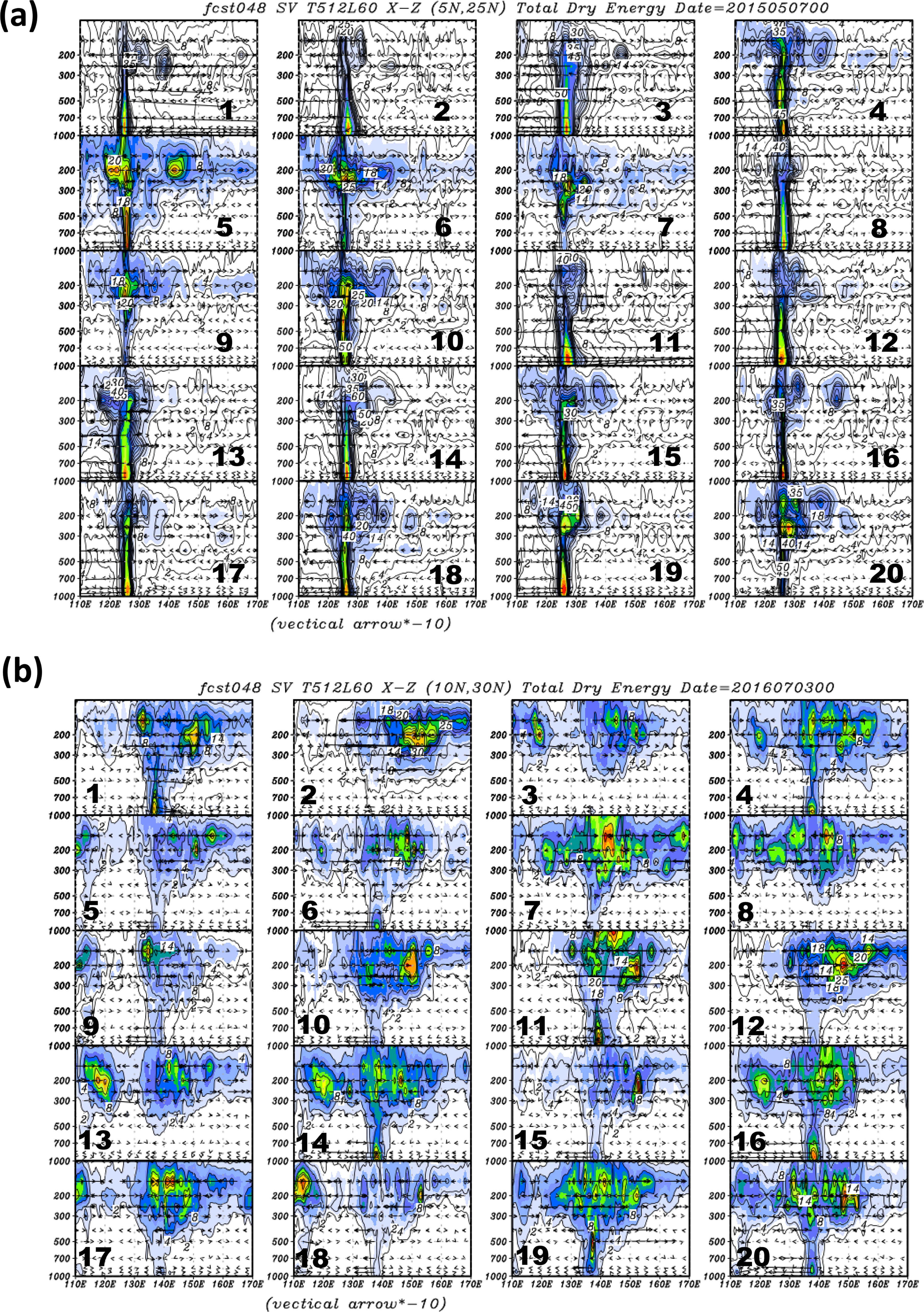
Fig. 6.
As in Fig. 4 (a) For the 48-hour forecast of 0000 UTC 7 May 2015, the valid time on 0000 UTC 9 May 2015. (b) For the 48-hour forecast of 0000 UTC 3 July 2016, the valid for 0000 UTC 5 July 2016.
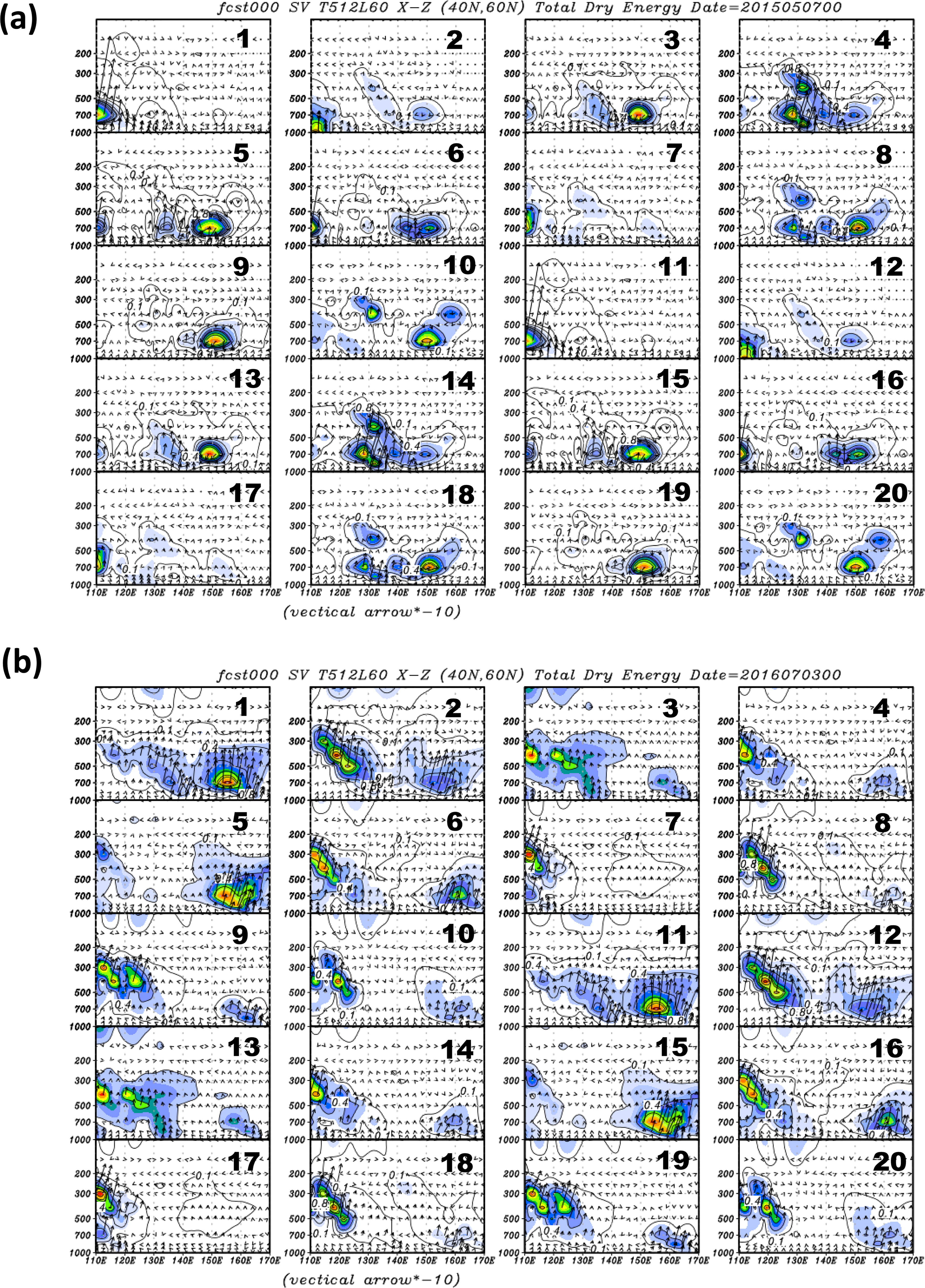
Fig. 7.
As in Fig. 4, but the mid-latitude singular perturbations are shown, and the latitudinal average is taken from to (a) For 0000 UTC 7 May 2015. (b) For 0000 UTC 3 July 2016.
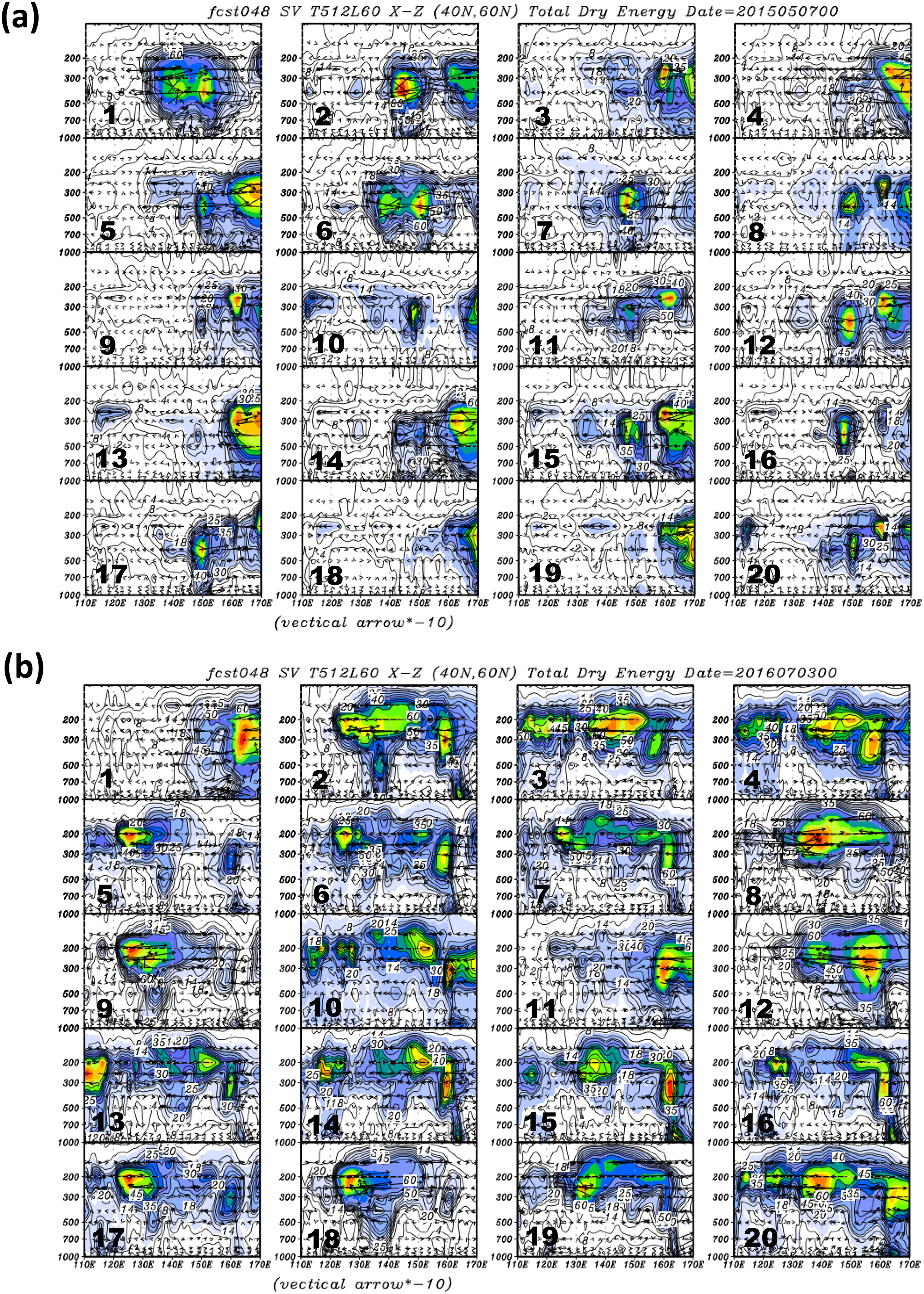
Fig. 8.
As in Fig. 7, but the forecasts of the mid-latitude singular vector perturbations are shown. (a) For 48-hour forecast of 0000 UTC 7 May 2015, the valid time 0000 UTC 9 May 2015. (b) For 48-hour forecast of 0000 UTC 3 July 2016, the valid time 0000 UTC 5 July 2016.
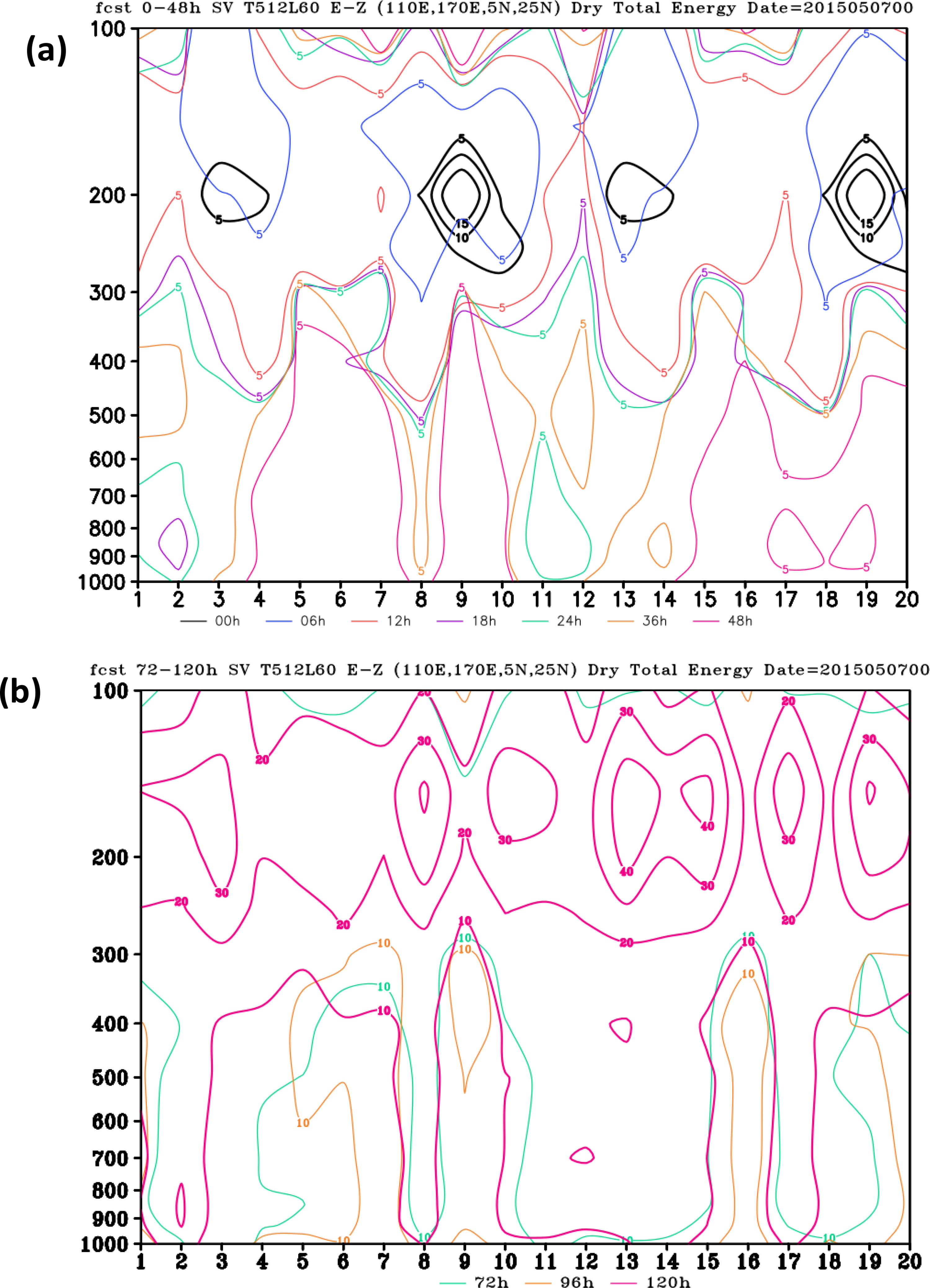
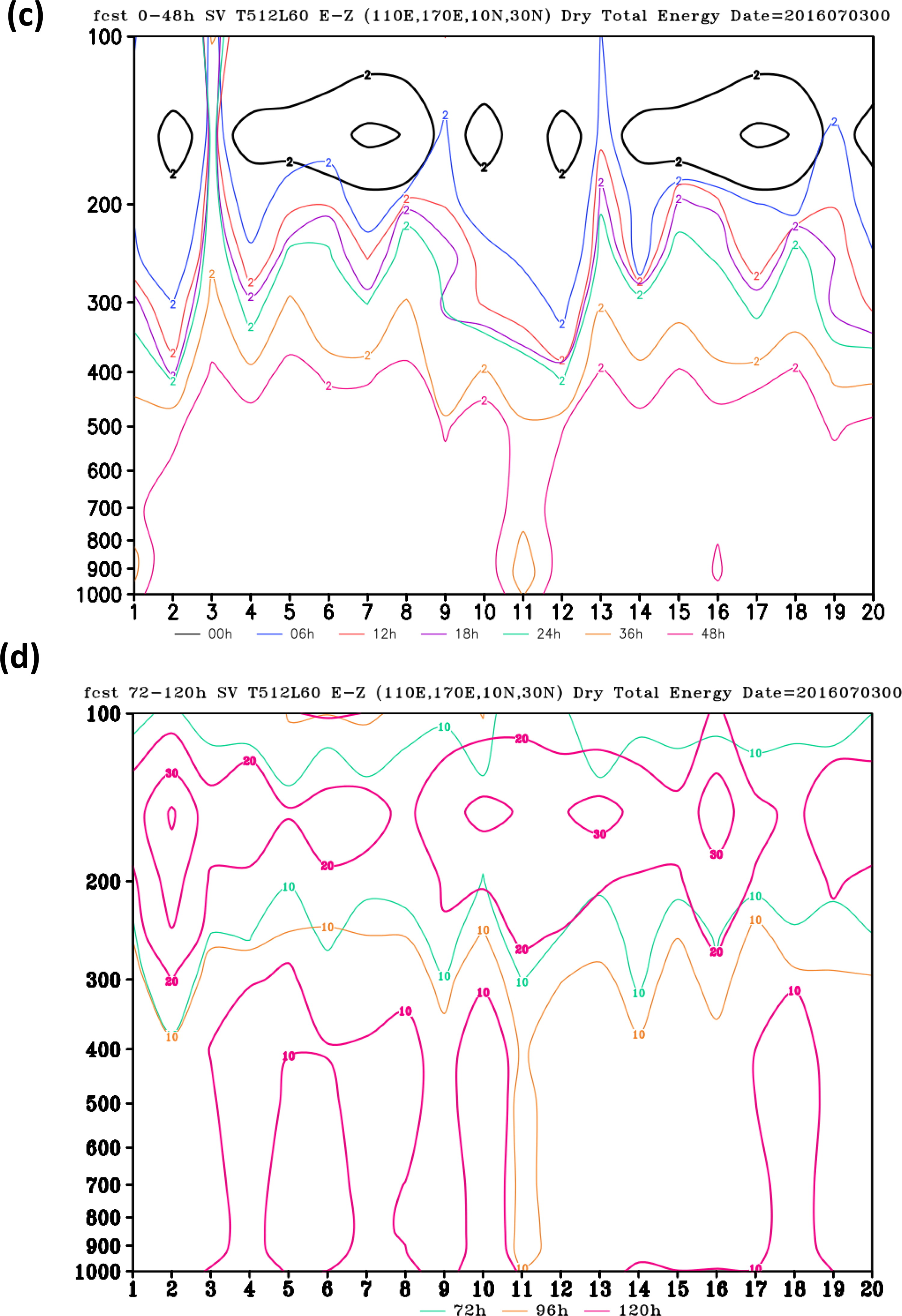
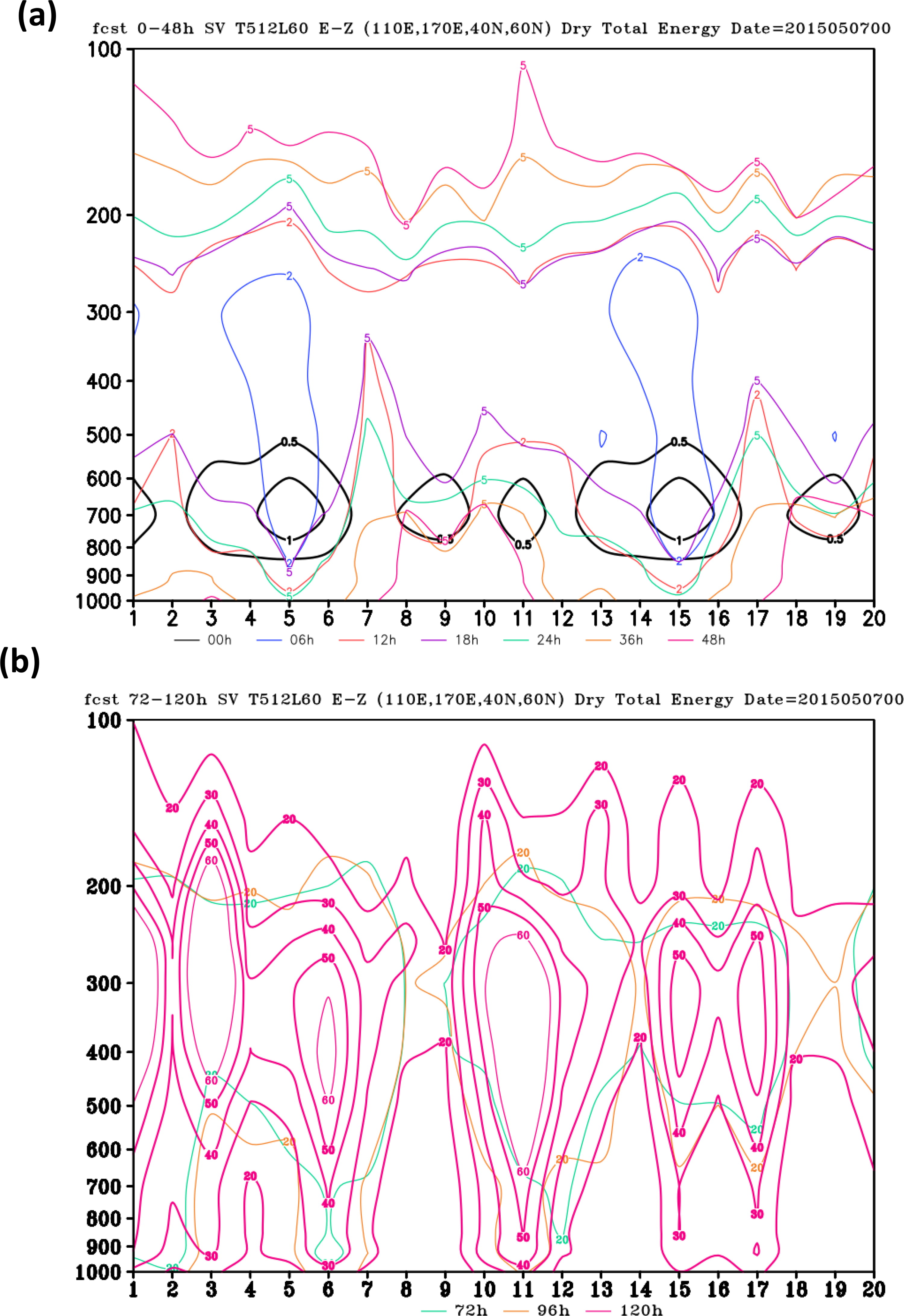
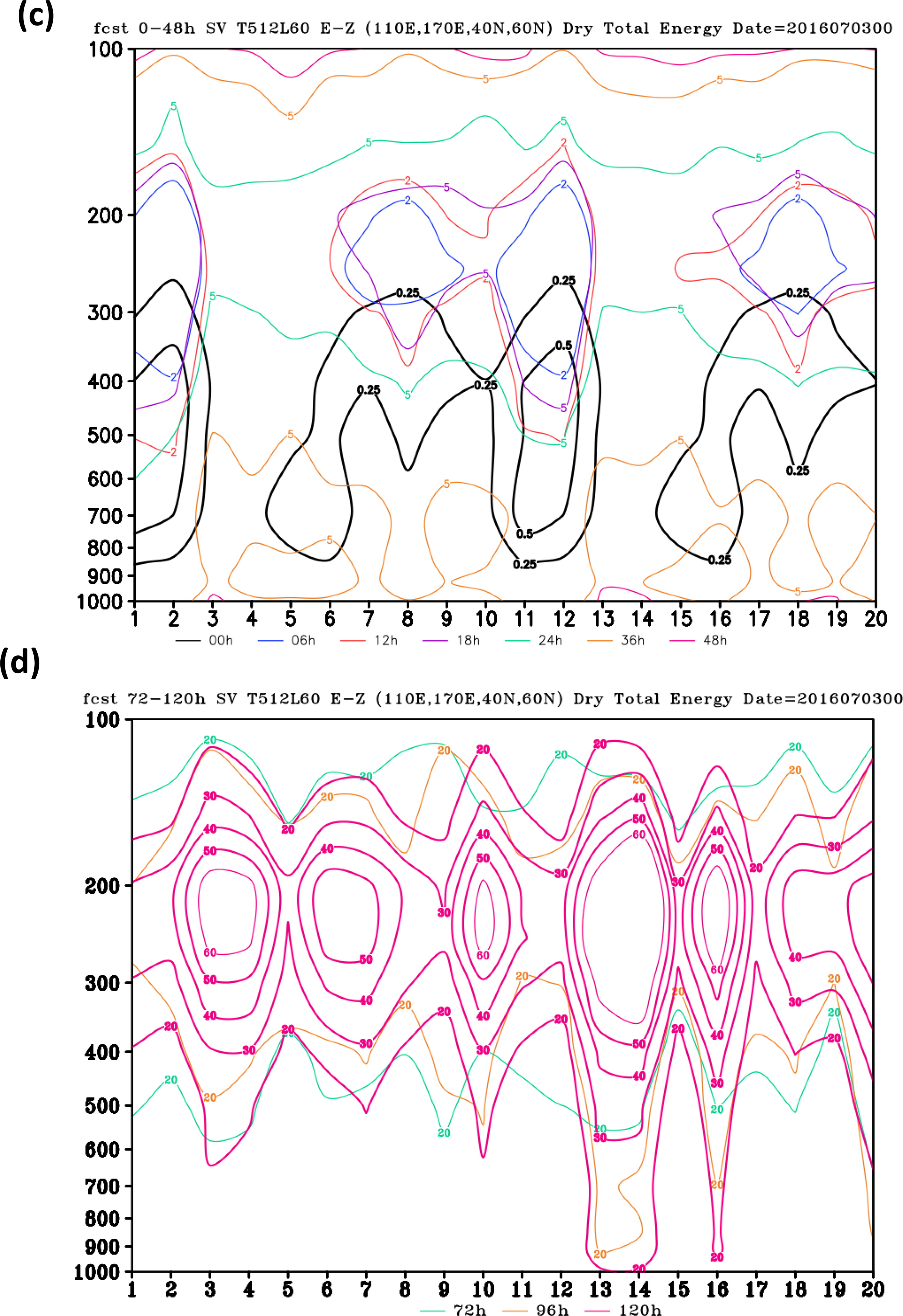
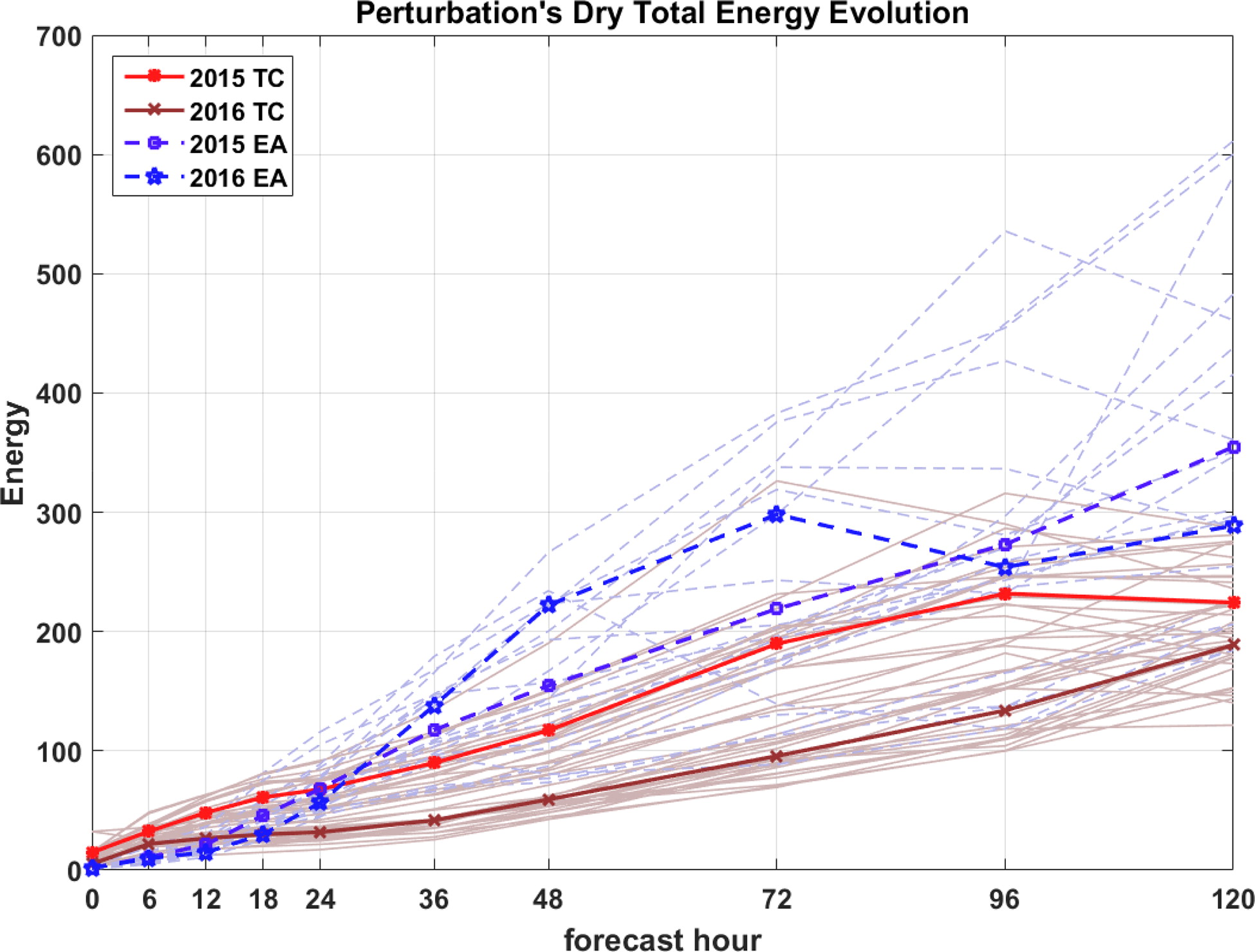
Fig. 11.
Time dependence of perturbation’s dry total energy (J/kg) for two cases in terms of both TC and East Asia domains. The total energy ensemble means of the TC domain (red solid lines) and East Asia domain (blue dashed lines) are shown. All the energy variations of ensemble members are indicated by grey solid lines (the TC domain) and grey dashed lines (East Asia domain).
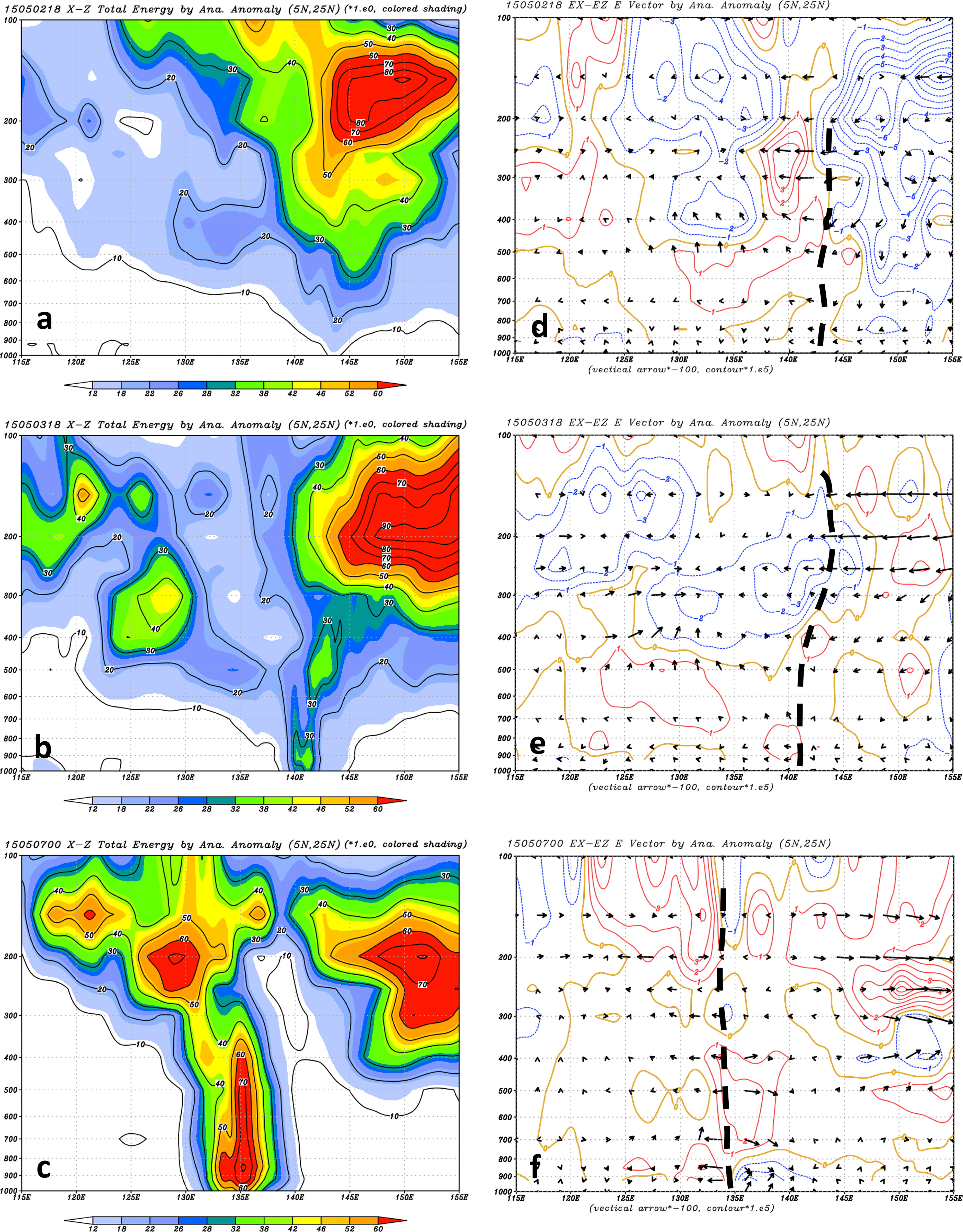
Fig. 12.
Structures of transient eddy dry total energy (J/kg) in analysis data are shown in longitude-pressure cross section. The latitudinal average is from to for Noul’s case. (a) 1800 UTC 2 May 2015, (b) 1800 UTC 3 May 2015, and (c) 0000 UTC 7 May 2015. The corresponding E-vector (x, p) components (arrow) and (contour) are shown in (d), (e), and (f). The thick dashed line marks the centre of the TC.
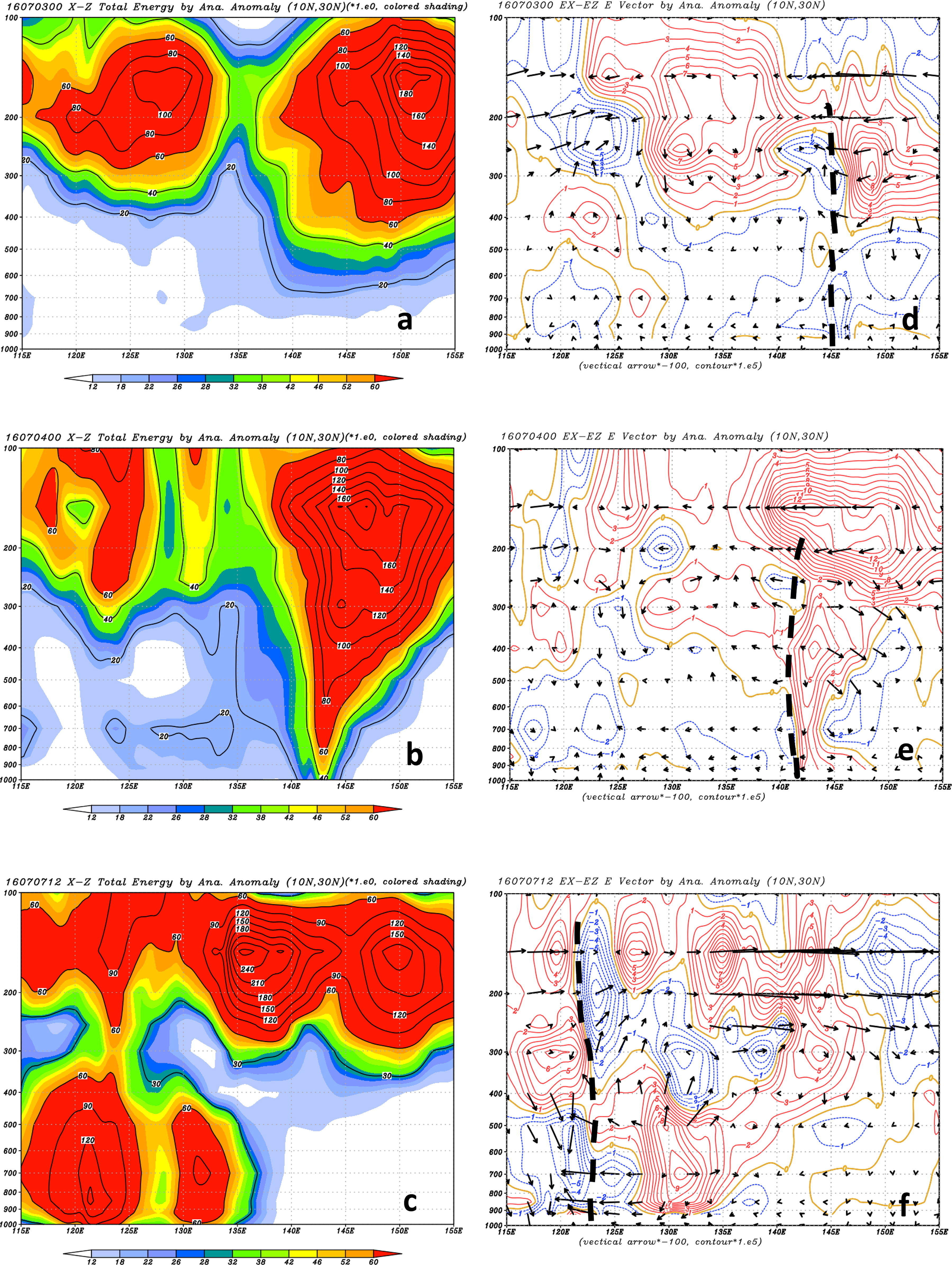
Fig. 13.
As in Fig. 12, but for Nepartak’s case. The latitudinal average is from to (a) 0000 UTC 3 July 2016, (b) 0000 UTC 4 July 2016, (c) 1200 UTC 7 July 2016. The corresponding E-vector (x, p) components (arrow) and (contour) are shown in (d), (e), and (f). The thick dashed line marks the centre of the TC.
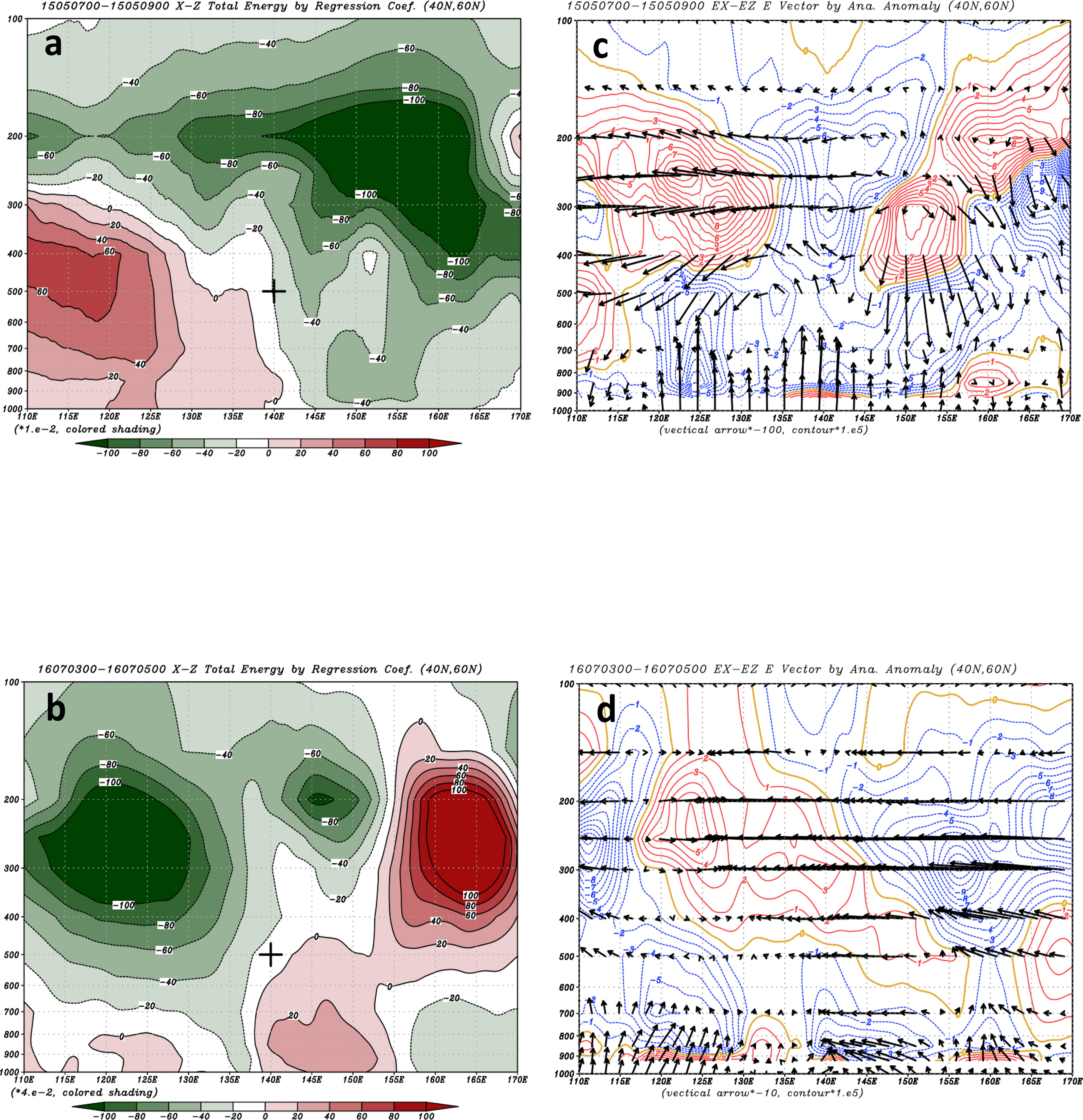
Fig. 14.
As in Fig. 12, but for the regression coefficients of the mid-latitude transient eddy dry energy. (a) The two days 0000 UTC 7 May 2015 − 0000 UTC 9 May 2015 average in Noul’s case, and (b) the two days 0000 UTC 3 July 2016 − 0000 UTC 5 July 2016 average in Nepartak’s case. The corresponding E-vector (x, p) components (arrow) and (contour) are shown in (c) and (d).
Table 2.
The comparisons between singular vector and transient eddy.
pillar in 48-hourupper layer development earlier than lower layer
singular vector in East Asia domain
cashew-nut
westward phase tilt
from lower layer to upper layer transient eddy around TC area
irregular round or comma sign*
pillar or funnel
from upper to lower layertransient eddy in mid-latitudewave train*wave trainlower layer upward
middle layer downward