
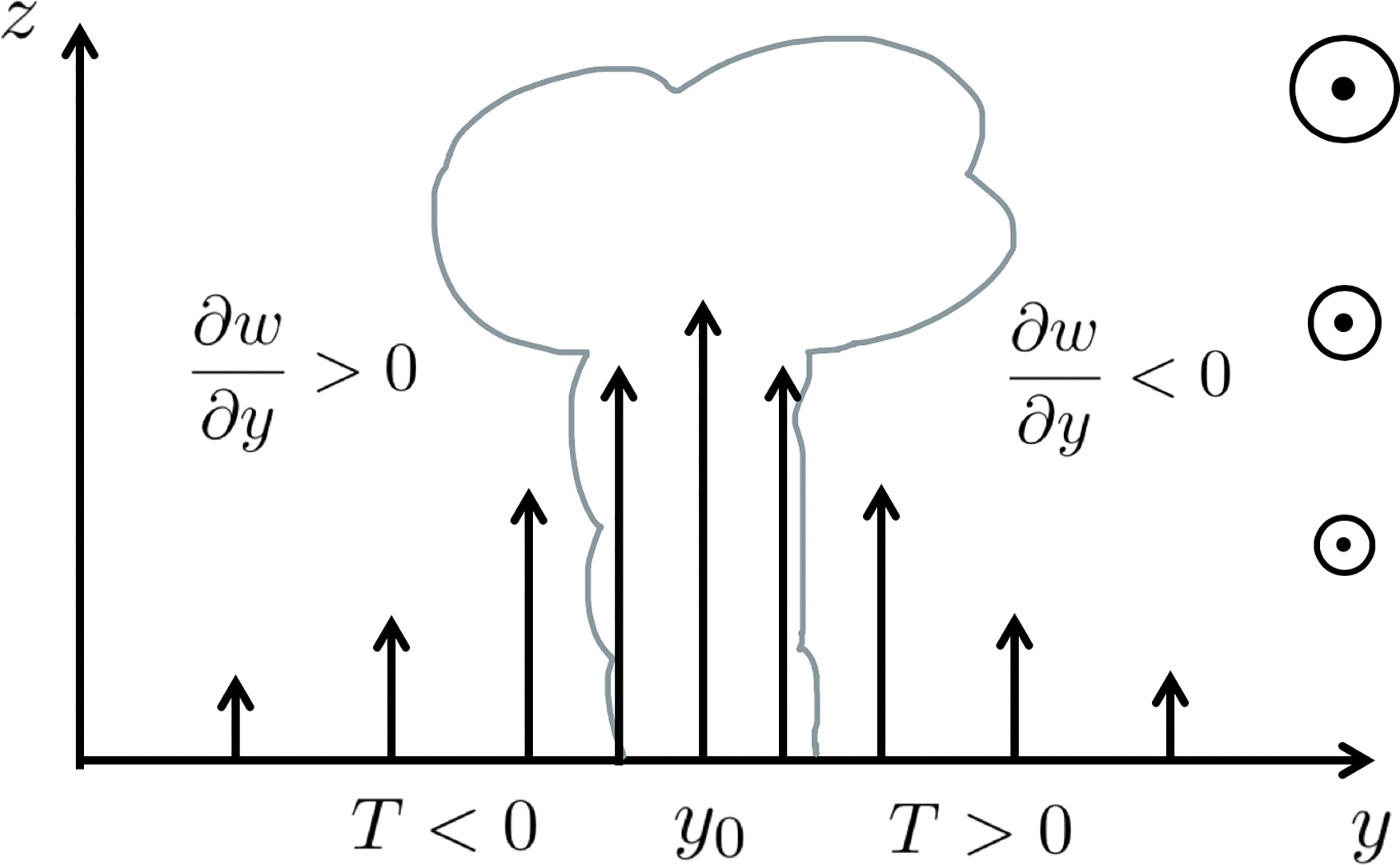
Fig. 1.
A sketch of a convective cloud. The black arrows show the updraft.
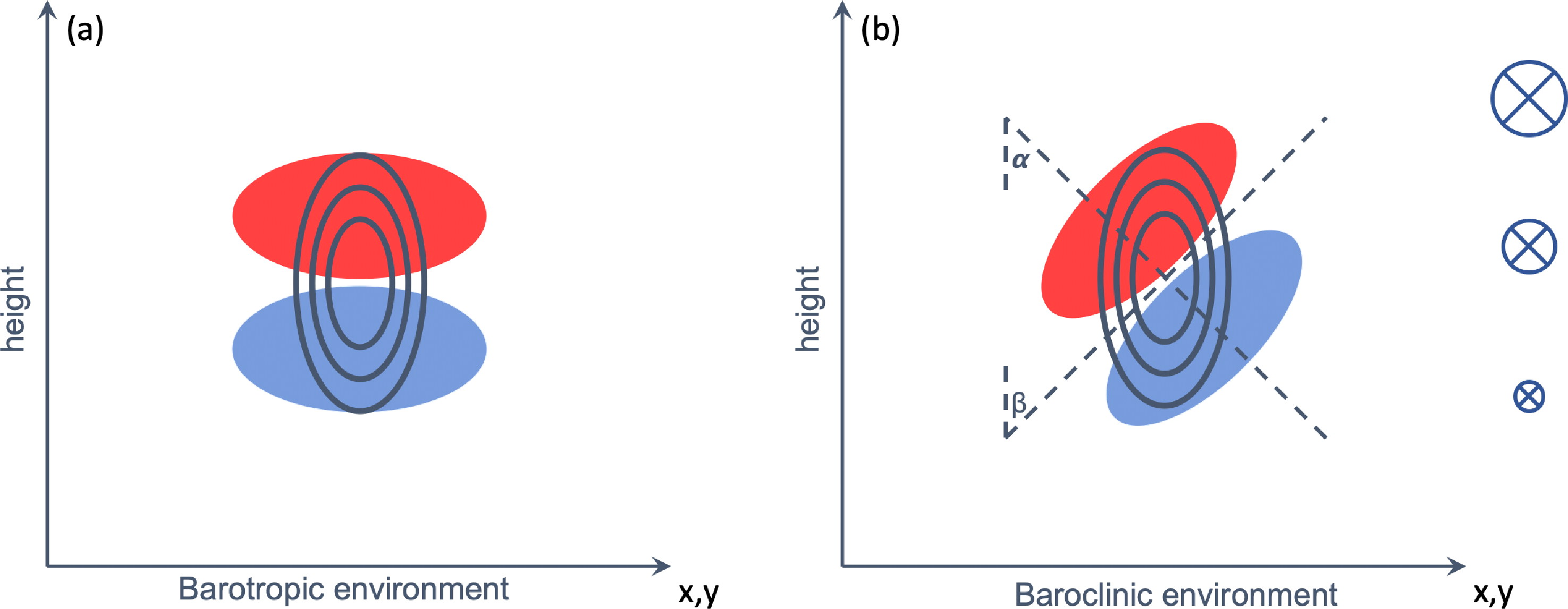
Fig. 2.
(a) Shows a sketch of the vertical PV dipole caused by heating for a barotropic environment. (b) Indicates the tilt of the dipole caused by the horizontal gradient of the vertical velocity and by the vertical change of the horizontal velocity. The red region indicates the positive pole and the blue region shows the positive pole. The figures are adapted from Chagnon and Gray (2009).
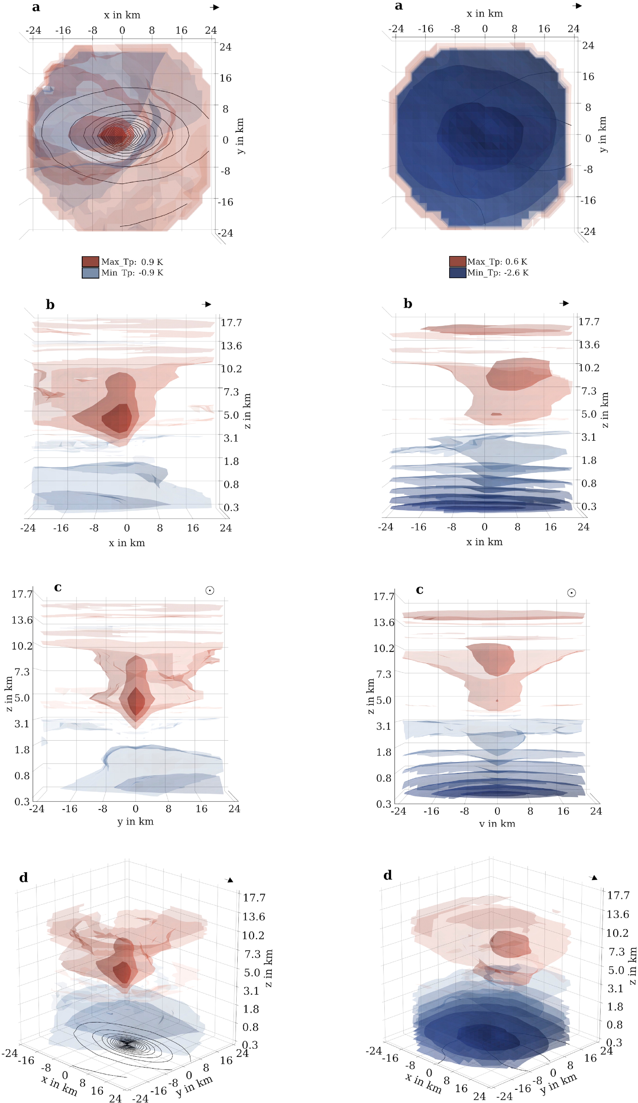
Fig. 3.
The anomaly composites of the potential temperature for intensity class D for the time (first column) and (second column) are shown. The rows are the different perspectives a, b, c and d. and denote the maximal and minimal value of the potential temperature anomaly in the troposphere. The red/blue isosurfaces mark the positive/negative values, where the isosurfaces become darker as the absolute values increase. The black contours show the precipitation sum of the next hour in 2 mm/h intervals.
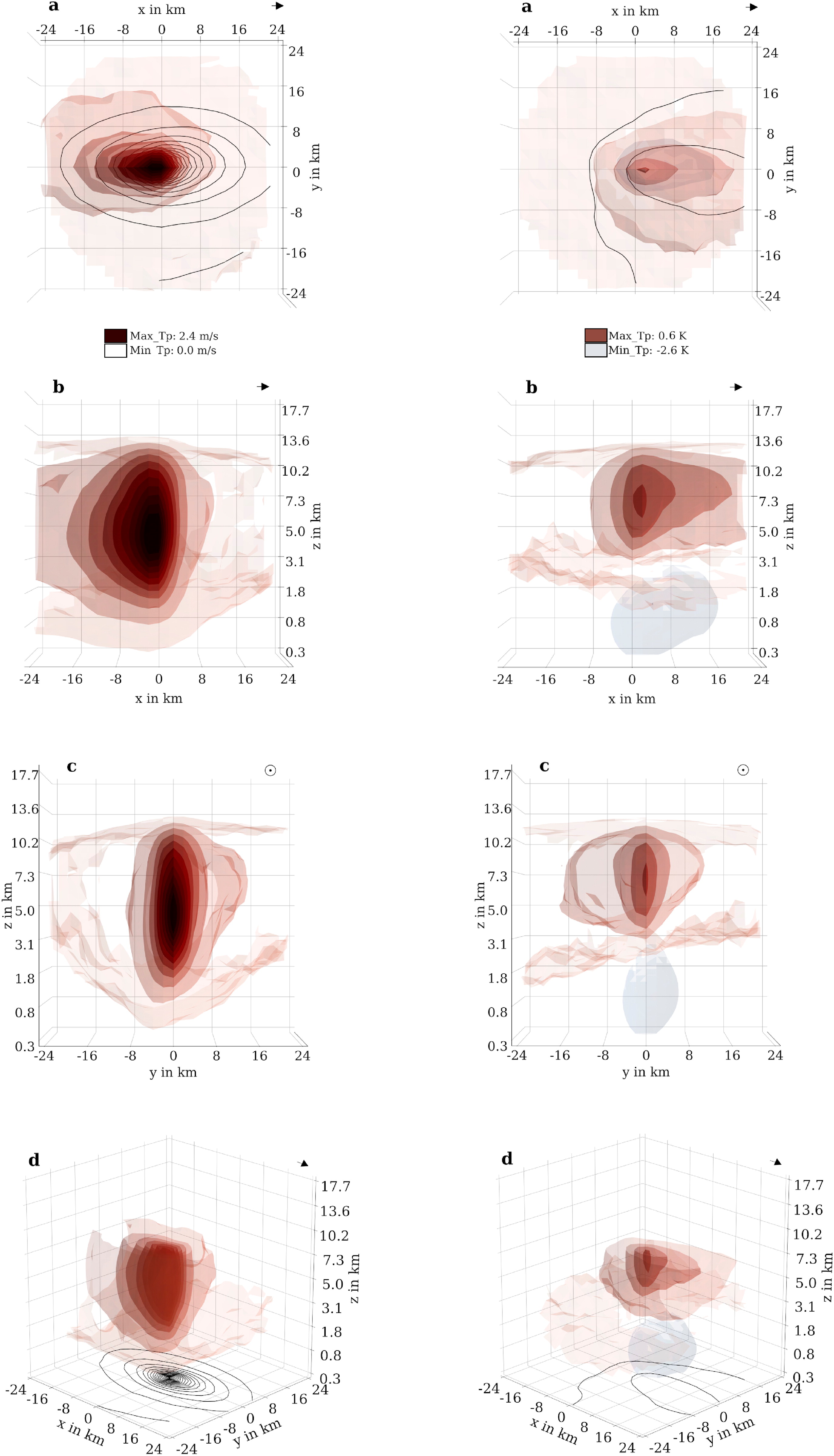
Fig. 4.
The composites of the vertical velocity for intensity class D for the time steps (first column) and tmax (second column) are illustrated, where the rows are the different perspectives a, b, c and d. and denote the maximal and minimal vertical velocity in the troposphere. The red/blue isosurfaces mark the positive/negative values, where the isosurfaces become darker as the absolute values increase. The black contours show the precipitation sum of the next hour in 2 mm/h intervals.
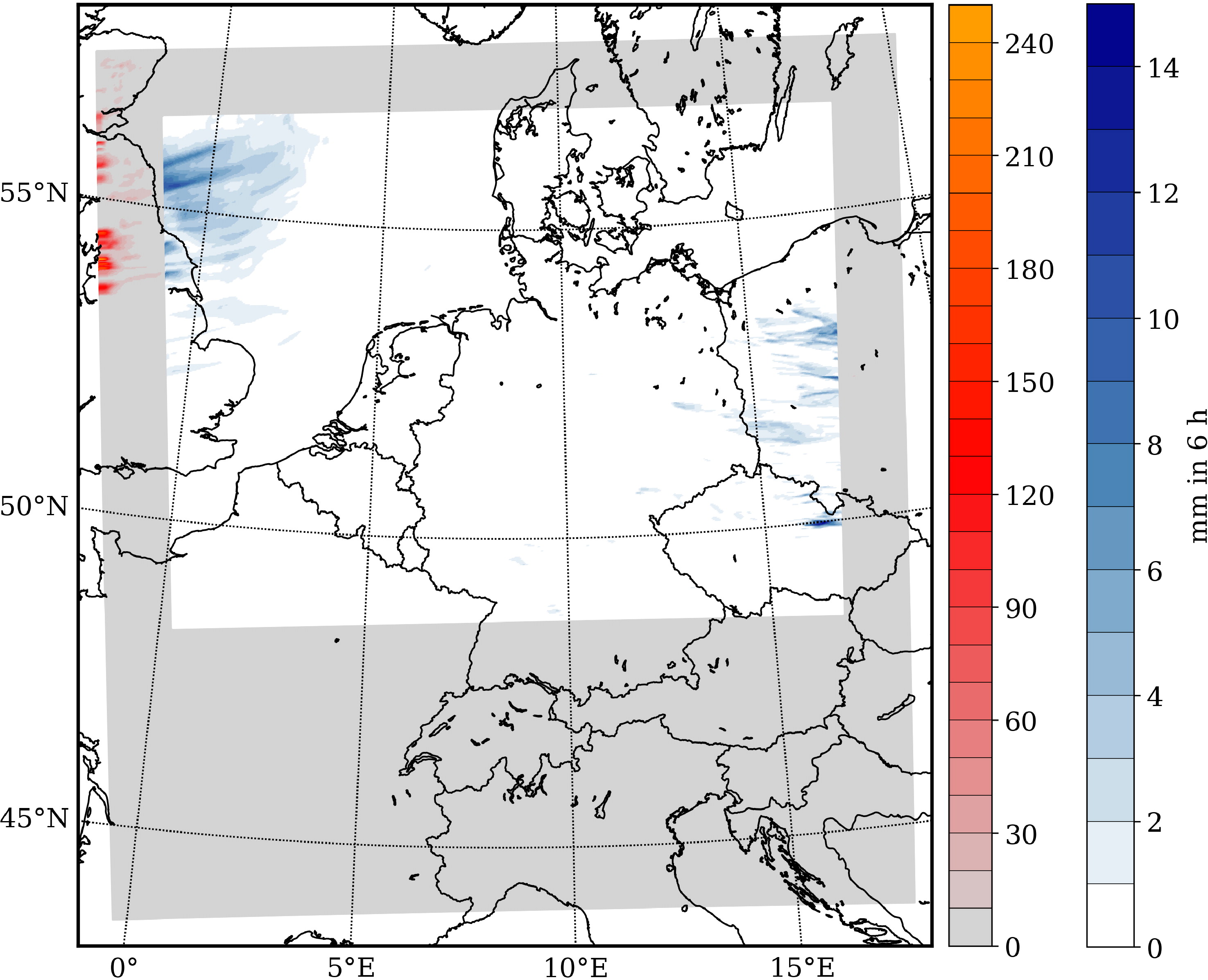
Fig. 5.
The domain of the COSMO-REA2 data set (gray box) and the data domain analyzed here (inner white box). The blue colorbar shows the precipitation (6 h-sum) from 29.06.2007 at 0:00 UTC with respect to the inner domain. The red colorbar shows the precipitation inside the gray box.
Table 1.
The intensity classes with respect to the precipitation intensity.
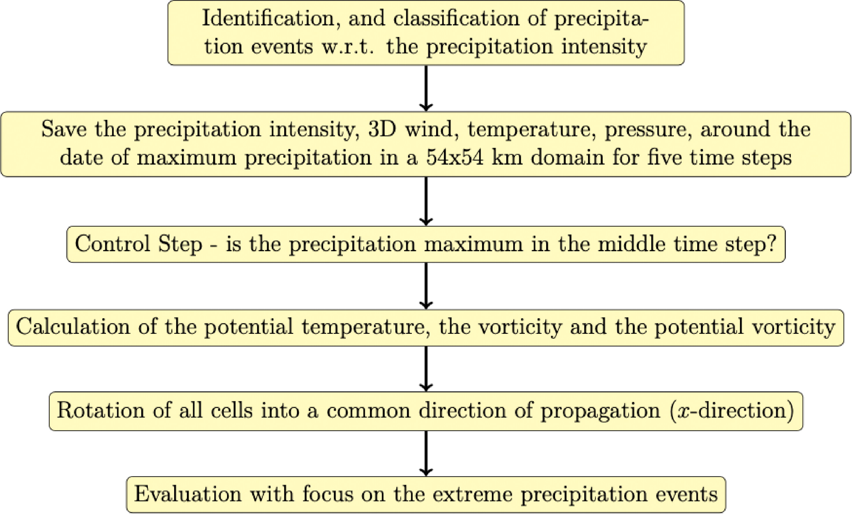
Fig. 6.
The steps to identify and calculate the 3D composites of the PV and the related variables during intense precipitation events are summarized. The categories of the precipitation intensities are listed in Table 1.
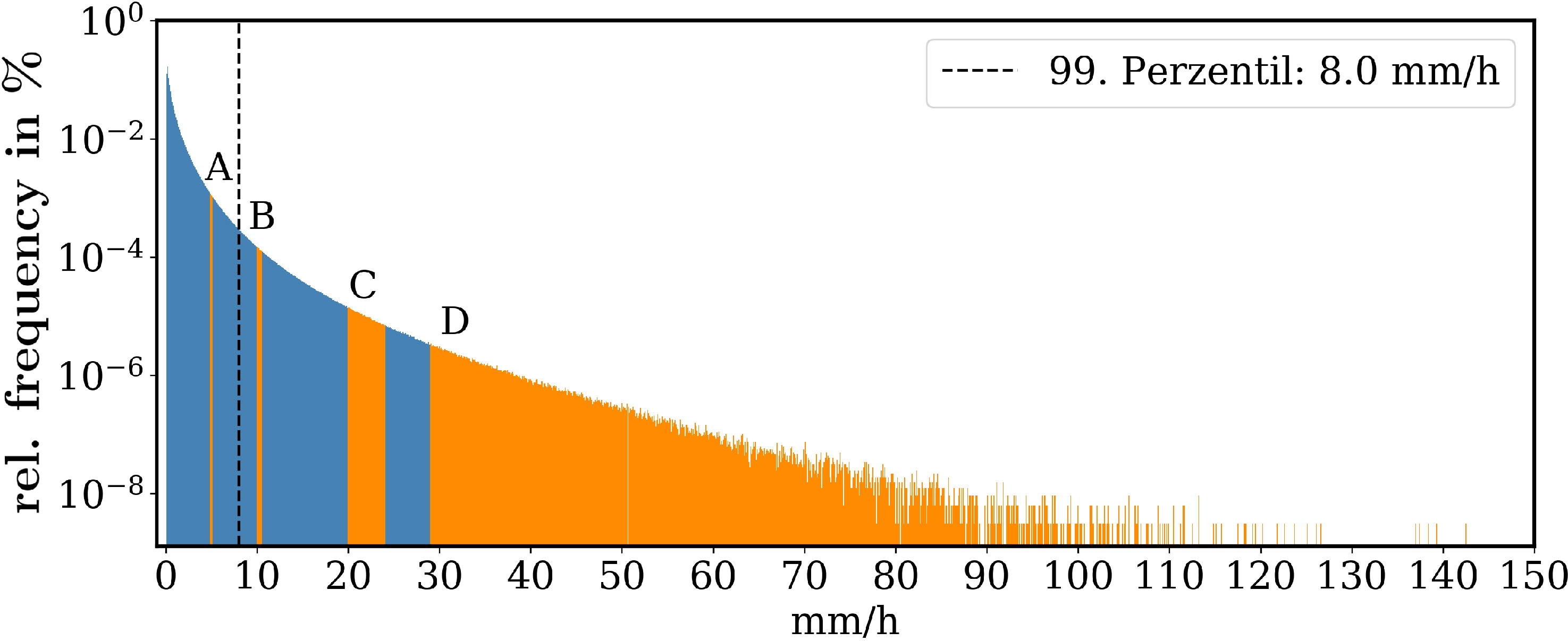
Fig. 7.
Relative frequency (logarithmic profile) of a precipitation intensity larger than 0.1 mm/h (blue) and the percentiles of the intensity classes of Table 1 (orange). The black dashed lines shows the 99. percentile.
Table 2.
The variables given at the selected points of time. The maximum precipitation intensity is at tmax.
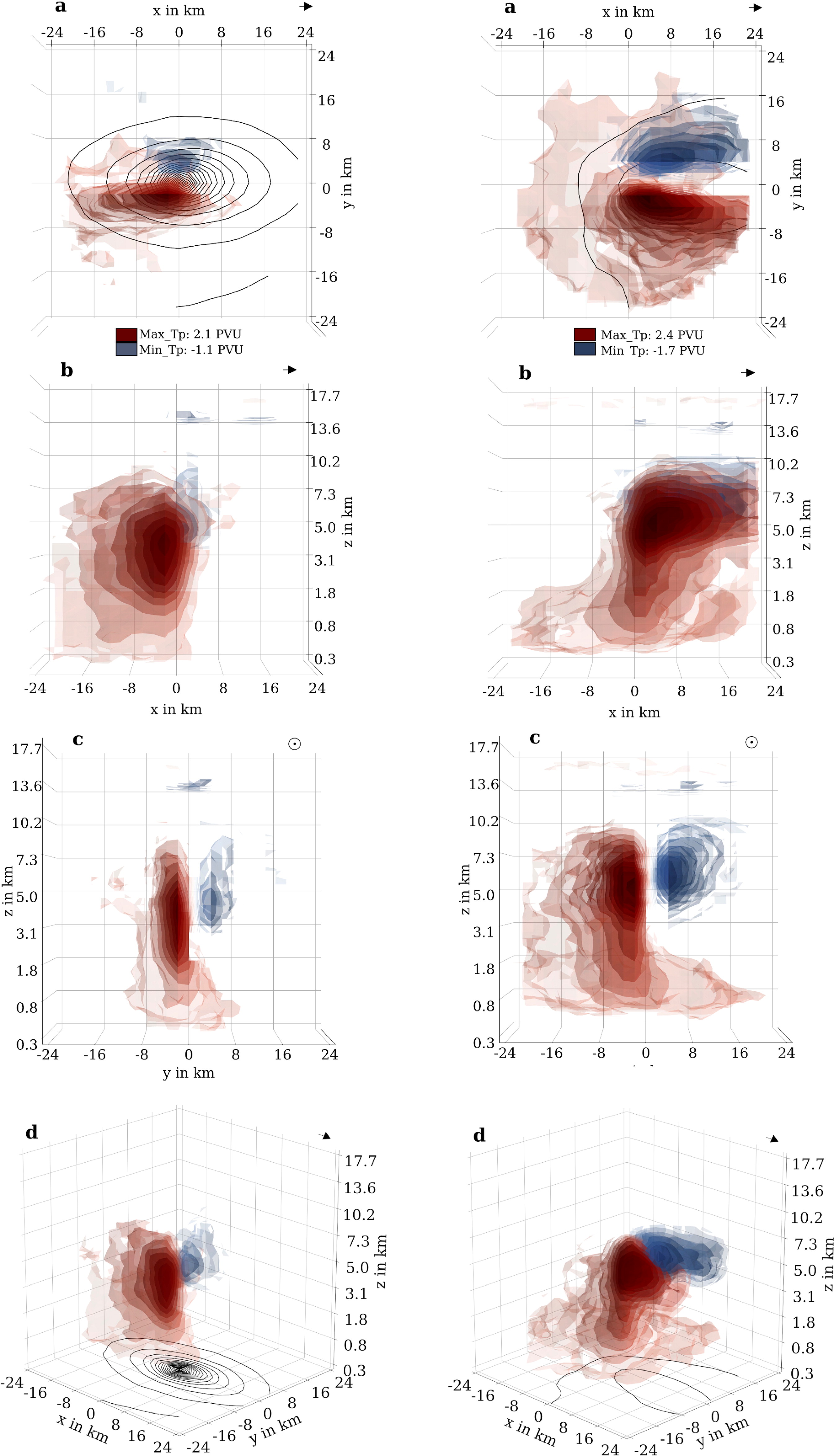
Fig. 8.
Composites of the relative PV for intensity class D for the time one hour before the maximal precipitation intensity ( first column) and at the time of maximal precipitation intensity tmax (second column). The rows are the different perspectives a, b, c and d. and indicate the maximal and minimal value of the relative PV in the troposphere, where only values from the ground up to a height of 8.5 km were taken into account. Positive values of the variables are indicated by red isosurfaces, where the surfaces become darker as the values increase. Negative values are marked by blue isosurfaces, where the darkness increases, when the absolute values become higher. The black contours show the precipitation sum of the next hour in 2 mm/h intervals.
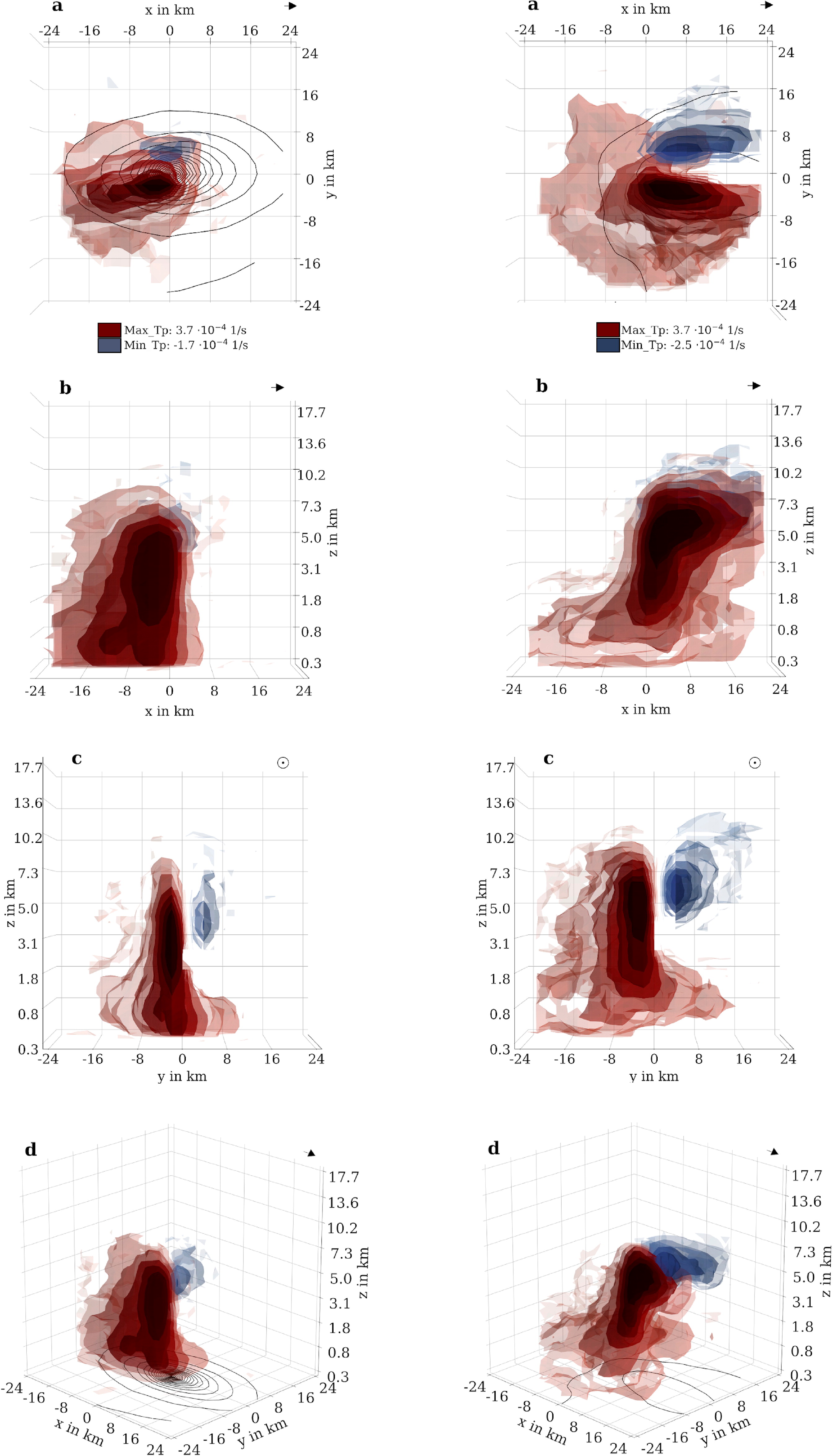
Fig. 9.
The first column shows the composites of the relative vorticity ζ for intensity class D at the time and the second columns shows the relative vorticity at the time tmax. The rows are the different perspectives a, b, c and d. and denote the maximal and minimal value of the vorticity in the troposphere. Red/blue isosurfaces mark the positive/negative values, where the isosurfaces become darker as the absolute values increase. The black contours show the precipitation sum of the next hour in 2 mm/h intervals.
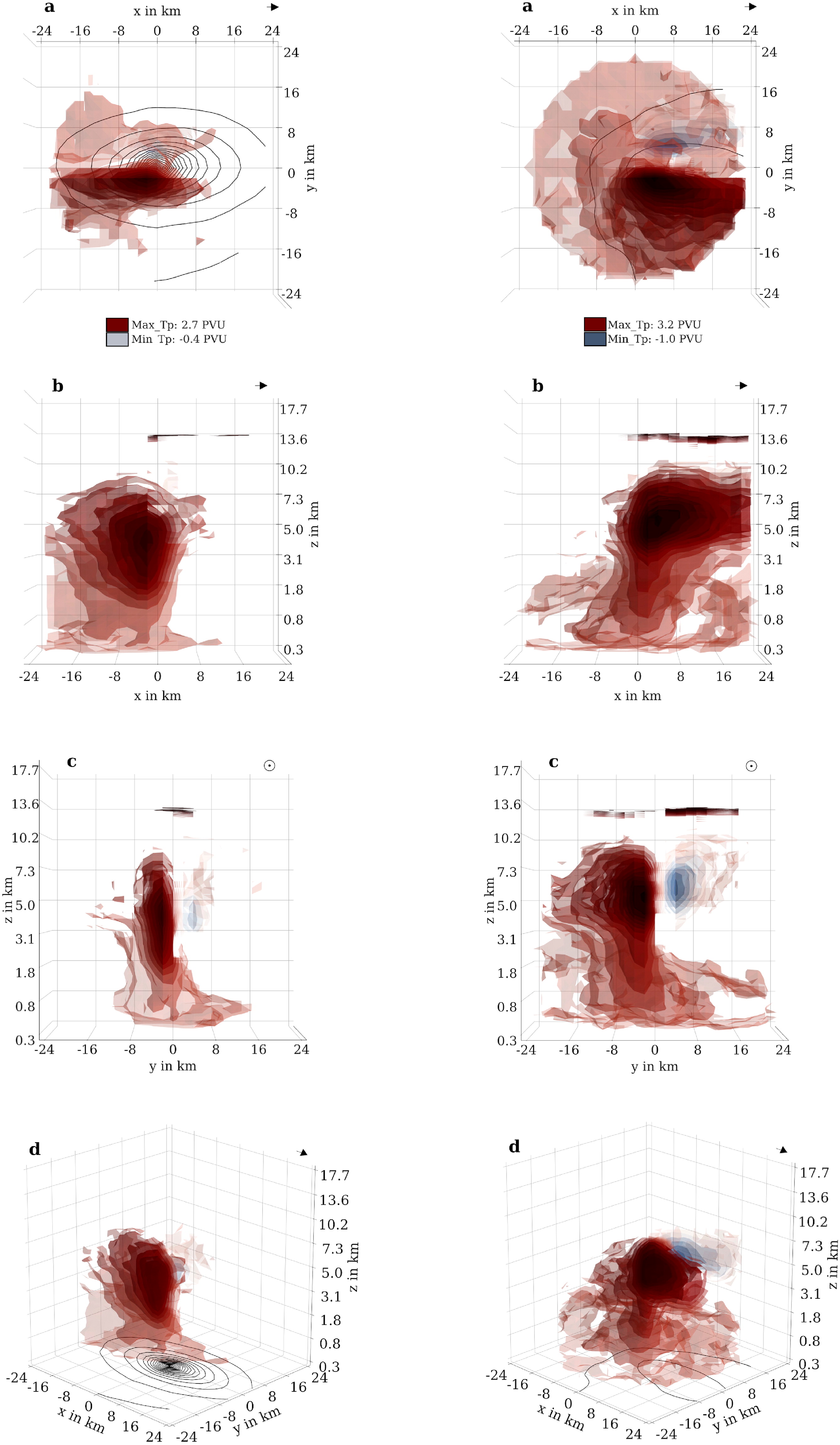
Fig. 10.
The composites of the absolute PV for intensity class D for the time steps (first column) and tmax (second column) are illustrated, where the rows are the different perspectives a, b, c and d. Here, and denote the maximal and minimal value of the absolute PV in the troposphere and as in the previous figures, the red/blue isosurfaces mark the positive/negative values, where the isosurfaces become darker as the absolute values increase. The black contours show the precipitation sum of the next hour in 2 mm/h intervals.
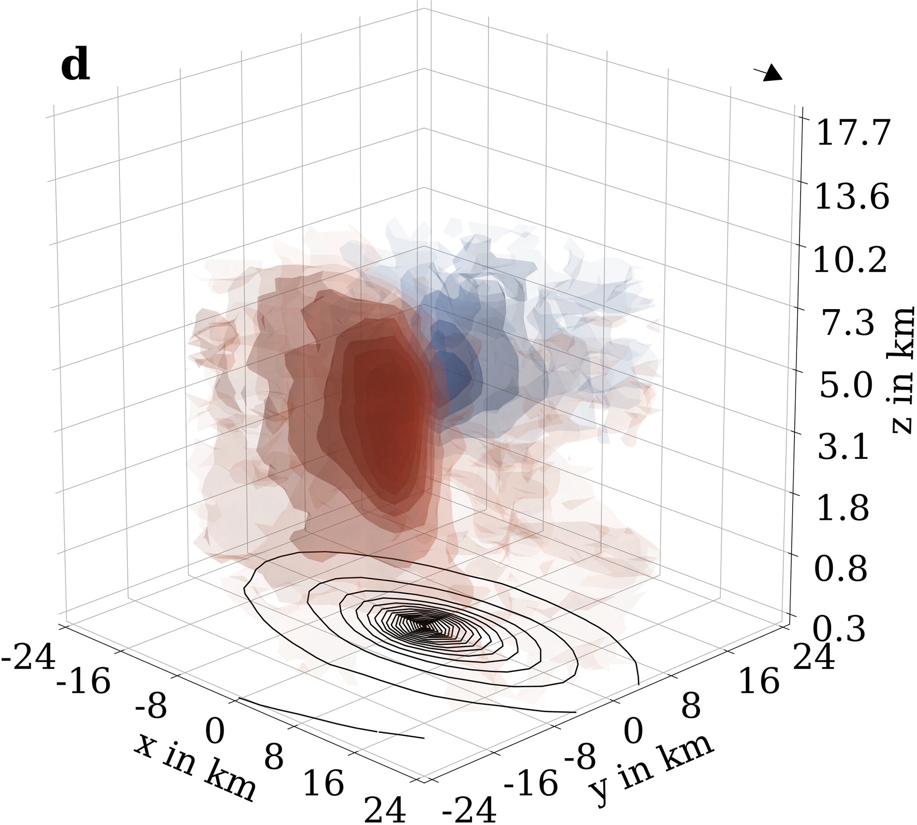
Fig. 11.
The relative PV composites of 3785 extreme precipitation events for the time step () is shown clearly indicating the horizontal dipole structure.
Table 3.
The maximal and minimal values of the potential vorticity with and without Coriolis parameter from the ground up to a height of 8.5 km.