
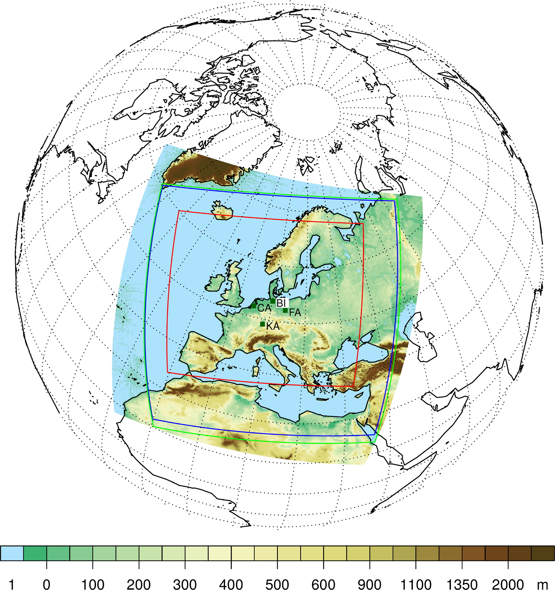
Fig. 1.
Model domains related to the different reanalyses and hindcasts (see Table 2). CCLM-oF is integrated within the red polygon, COSMO-REA6 within the blue polygon and UE-UKMO within the green polygon. The UE-SMHI domain is denoted by the orography map [m].
Table 1.
Location, boom height above ground [m], estimation of roughness [m] and data availability for 2006–2007 [%] at the sites considered for evaluation. The roughnesses for the observational sites are not extracted in a consistent way (turbulent flux measurements at different heights vs. Richardson methods). The values of the hindcasts are extracted from the grid morphology near the site location. The values from UE-UKMO are not part of the standard output due to tile-based calculation within land-surface model JULES (Best et al., 2011; Clark et al., 2011).
Table 2.
The models evaluated in this study. The PBL model levels are with respect to the lowest 1500 m. The positions of the model levels are related to flat terrain and to a surface pressure of 1013.26 hPa. For interpretation of the results, the datasets are indicated with the following abbreviations: CCLM-oF-SN, CCLM-oF, COSMO-REA6, UE-SMHI and UE-UKMO.
Table 3.
The static stability classes used for investigation. The classification is shown to be dependent on the vertical gradients of (potential) temperature. Moreover, the likelihood of occurrence [%] of static stability is listed for the flux towers.
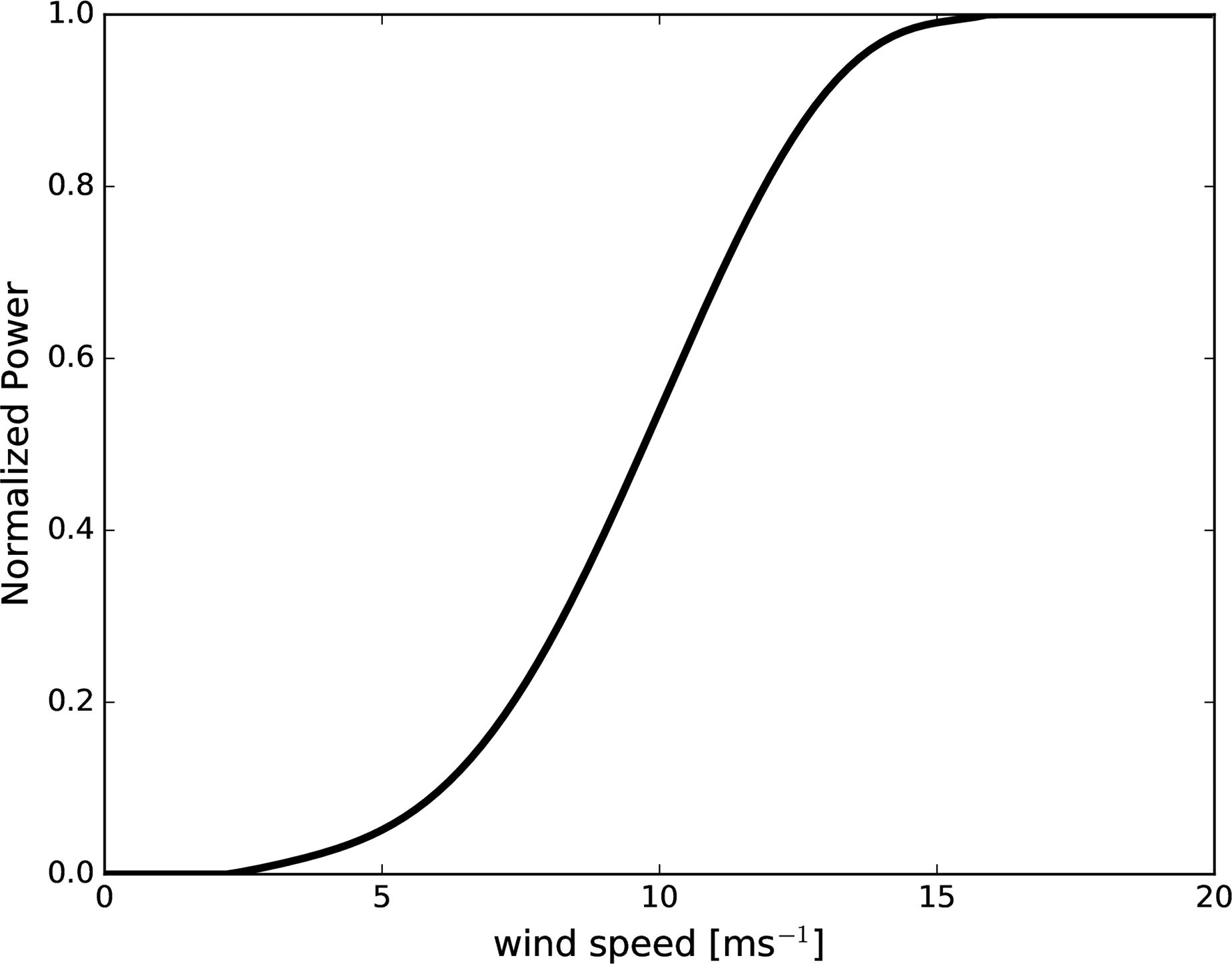
Fig. 2.
Characteristic power curve as given by the ENERCON E70 wind turbine (2310 kW, with a diameter of 70 m).
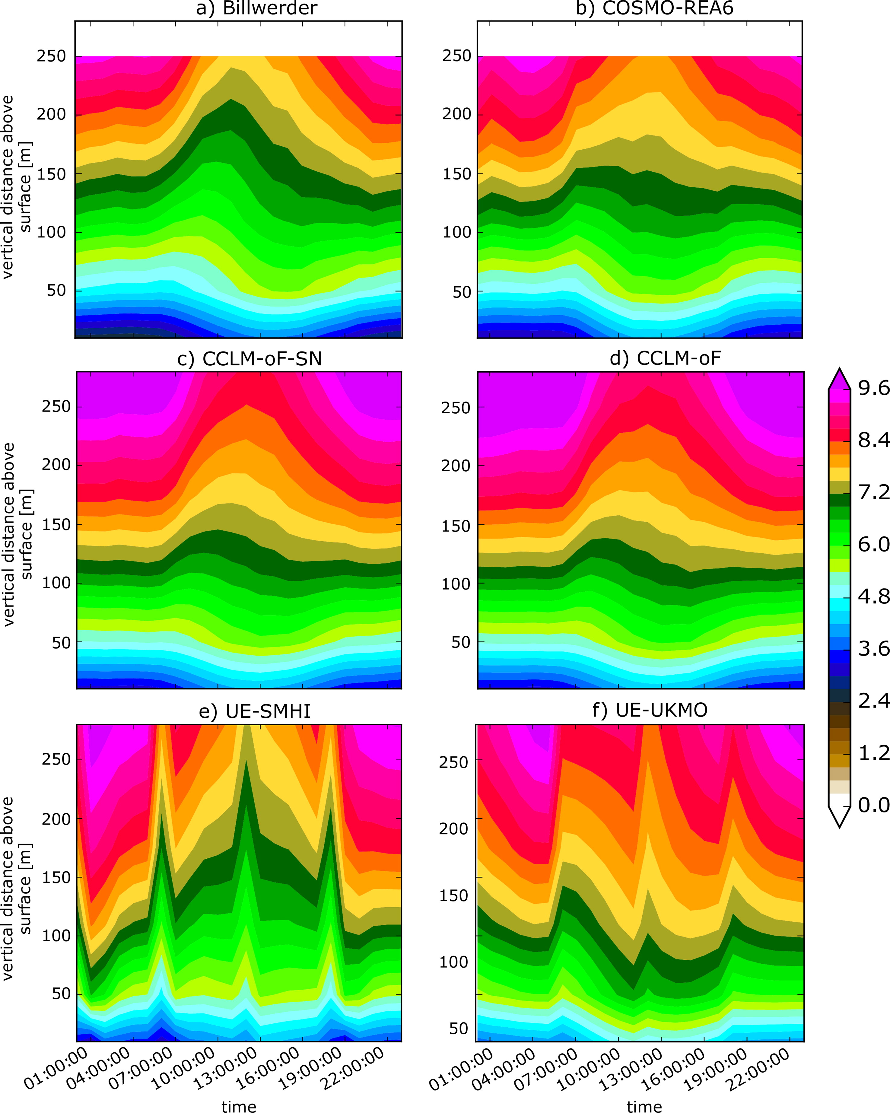
Fig. 3.
Hamburg, diurnal cycle of wind speed [m/s] (hourly values) for the whole year 2006–2007 for observation (a) and five different assimilation experiments (b–f). Note, that the data for COSMO-REA6 is not available above 250 m.
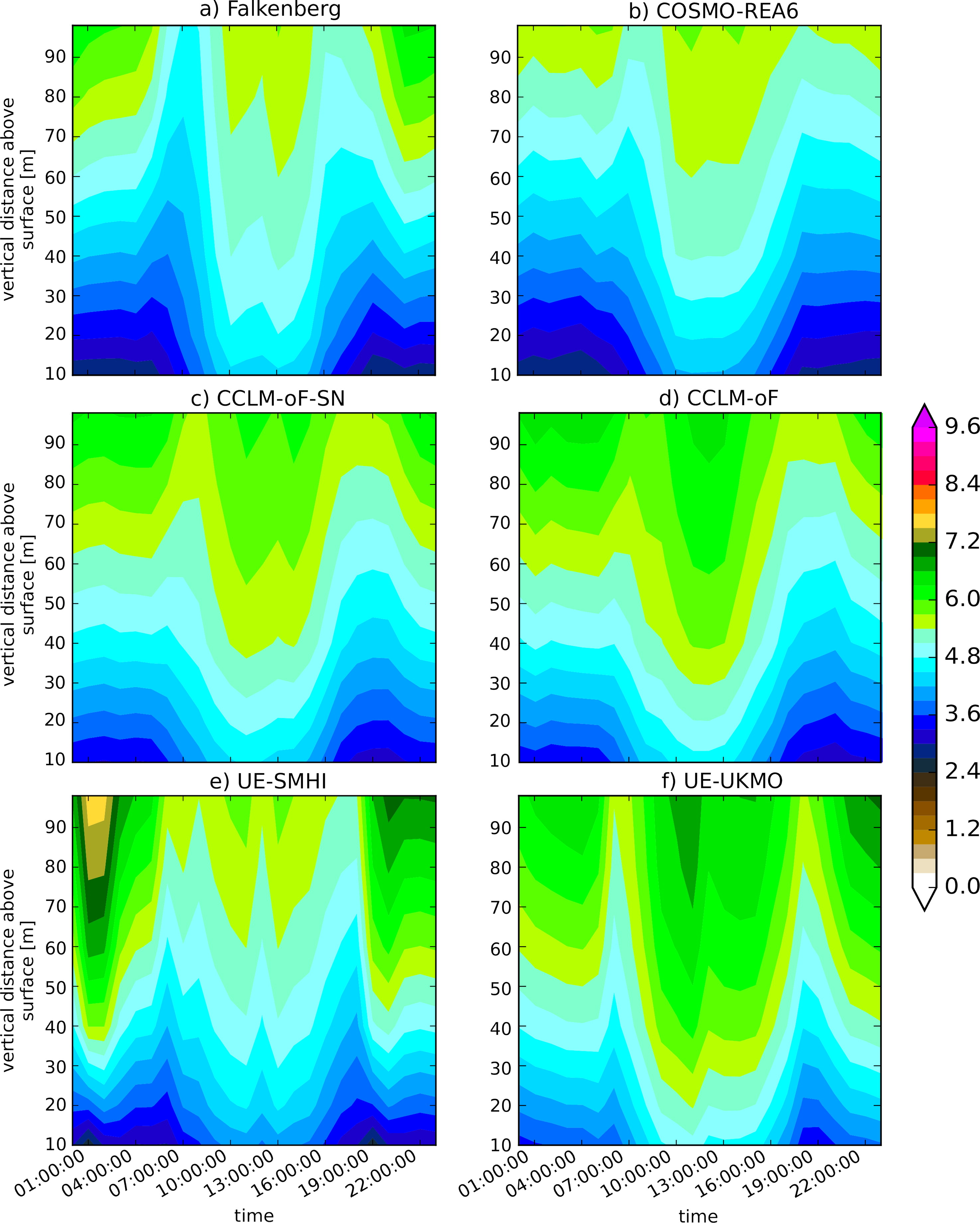
Fig. 4.
Same as Figure 3 but for the tower at Falkenberg and only for the months of May to September in 2006 and 2007.
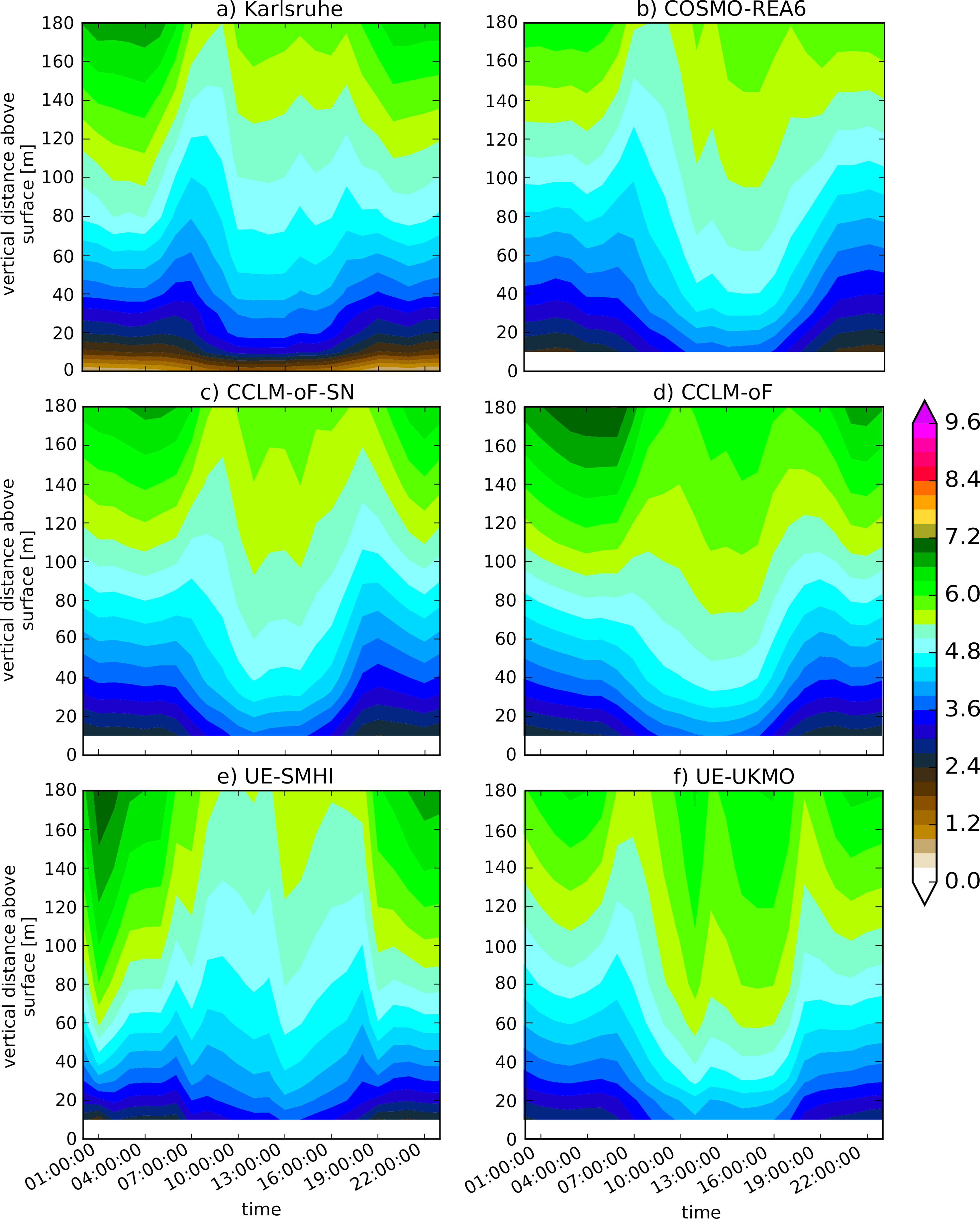
Fig. 5.
Same as Figure 3 but for the tower at Karlsruhe and only for the months of May to September in 2006 and 2007.
Table 4.
Kling-Gupta efficiency for the mean diurnal cycle in ‘MJJA’ (summer) and ‘NDJFM’ (winter). The towers are listed, and the heights are grouped for the near-surface, above 100 m and in between. The bold numbers indicate that the performance exceeds 0.4, which requires, for instance, and Model names are shortened by omitting the first part.
Table 5.
Estimation of the shape parameter (first number in each cell) and scale parameter (second number) of the Weibull distribution with respect to the selected measurement locations. Model names are shortened by omitting the first part. The ‘star’ indicates that the uncertainty of parameter estimation is larger than 0.1. In addition, EMD is given [m s−1].
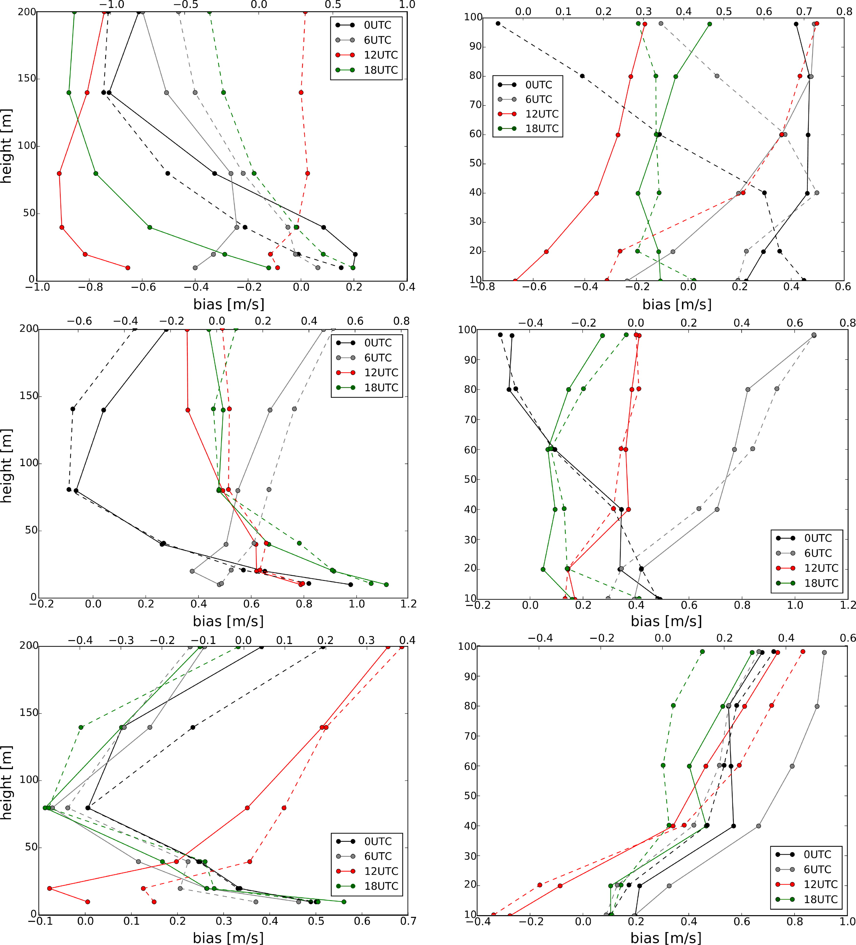
Fig. 6.
Median wind speed bias at 00, 06, 12 and 18 UTC at the towers Cabauw (left panel) and Falkenberg (right panel). Top: The UE-SMHI (solid lines, lower x-axis) and UE-UKMO reanalyses (dashed lines, upper x-axis) are shown with respect to the years 2006 and 2007 for summer. Middle: The same is shown but for CCLM-oF-SN (solid lines, lower x-axis) and COSMO-REA6 (dashed lines, upper x-axis). Bottom: The same is shown as in the middle panel but for winter.
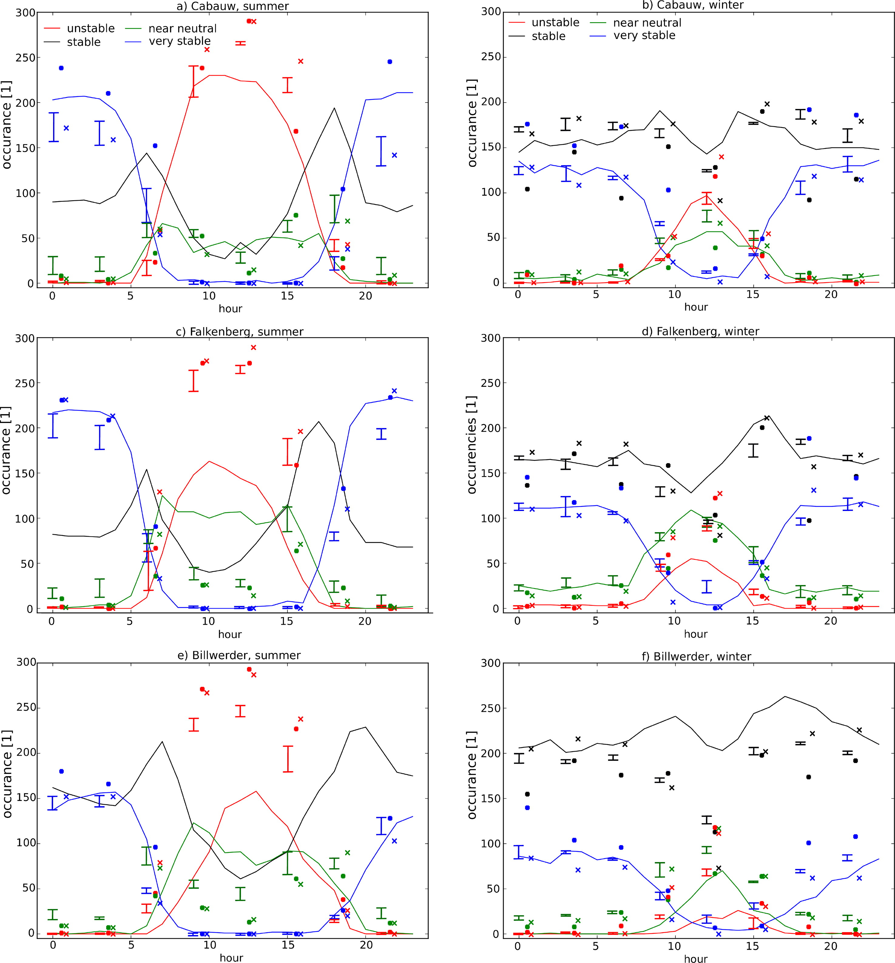
Fig. 7.
Diurnal cycle of occurrence of 4 different types of stratification (Table 3) for summer (‘MJJAS’, left) and winter (‘NDJFM’, right) and at towers Cabauw (a, b), Falkenberg (c, d) and Billwerder (e, f). The straight lines indicate the absolute frequency measured, and the symbols indicate the absolute frequencies simulated (‘x’: UE-UKMO, rectangle: UE-SMHI, range indicator: COSMO models). For readability, the simulated frequency of ‘st’ cases is shown only in winter. The colors belong to different stabilities (legend of the figures in the top row).
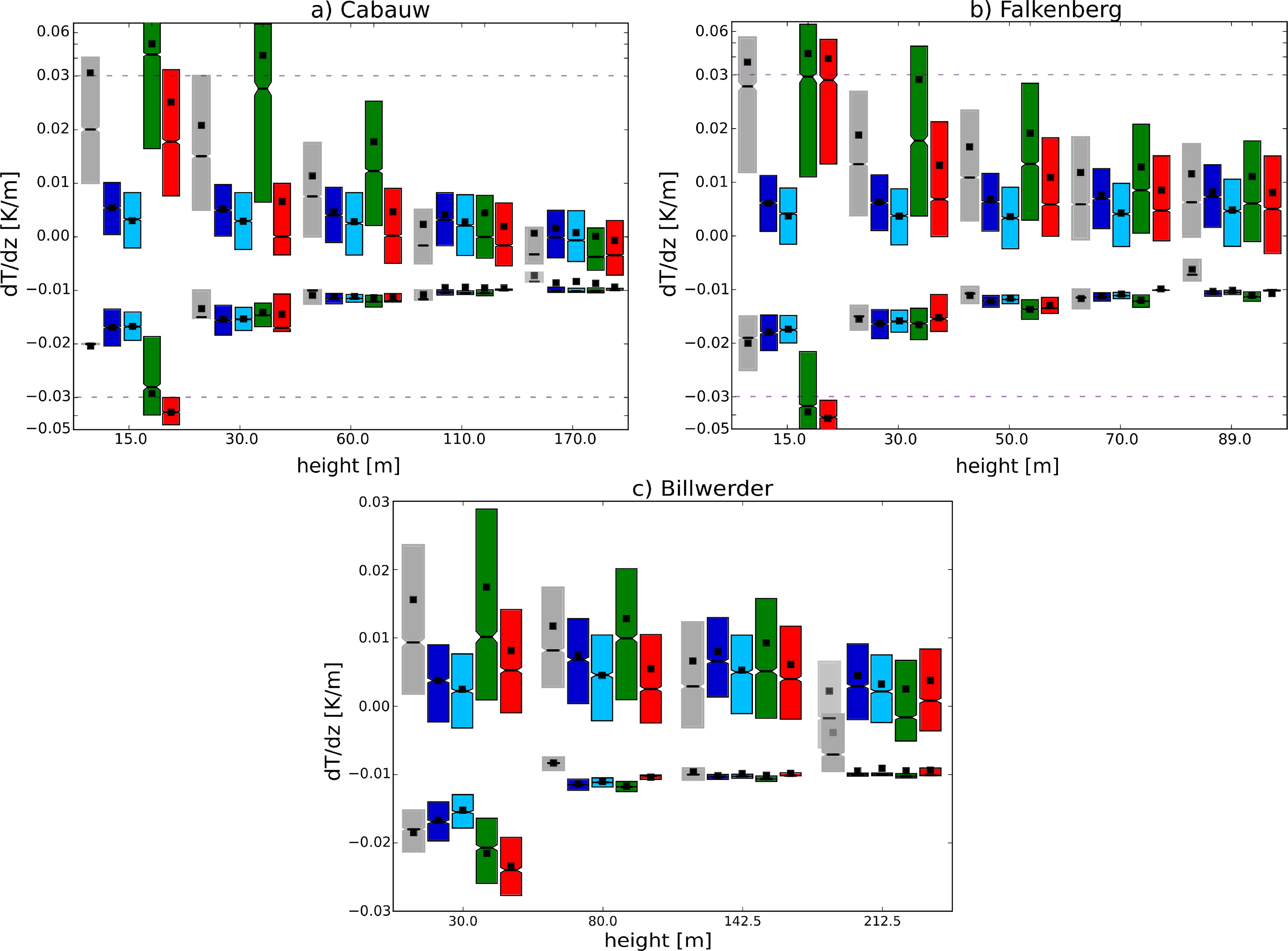
Fig. 8.
Temperature profiles depending on the stratification at Cabauw (a), Falkenberg (b) and Billwerder (c). Modified box plots are shown for the observations (gray), COSMO-REA6 (dark blue), CCLM-oF-SN (light blue), UE-SMHI (green) and UE-UKMO (red). The upper part of each figure refers to the very stable stratifications, and the lower part refers to the unstable stratifications. ‘Modified box plot’ means that only the upper and lower quartiles of the data are visualized by the box, and the median is indicated by the straight line in the box and the mean by the small black rectangle. Furthermore, transparency is used with the last gray boxes at Billwerder to distinguish between the data. Moreover, the horizontal dashed lines indicate the transition from a linear scale to a logarithmic scale (see the y-axis).
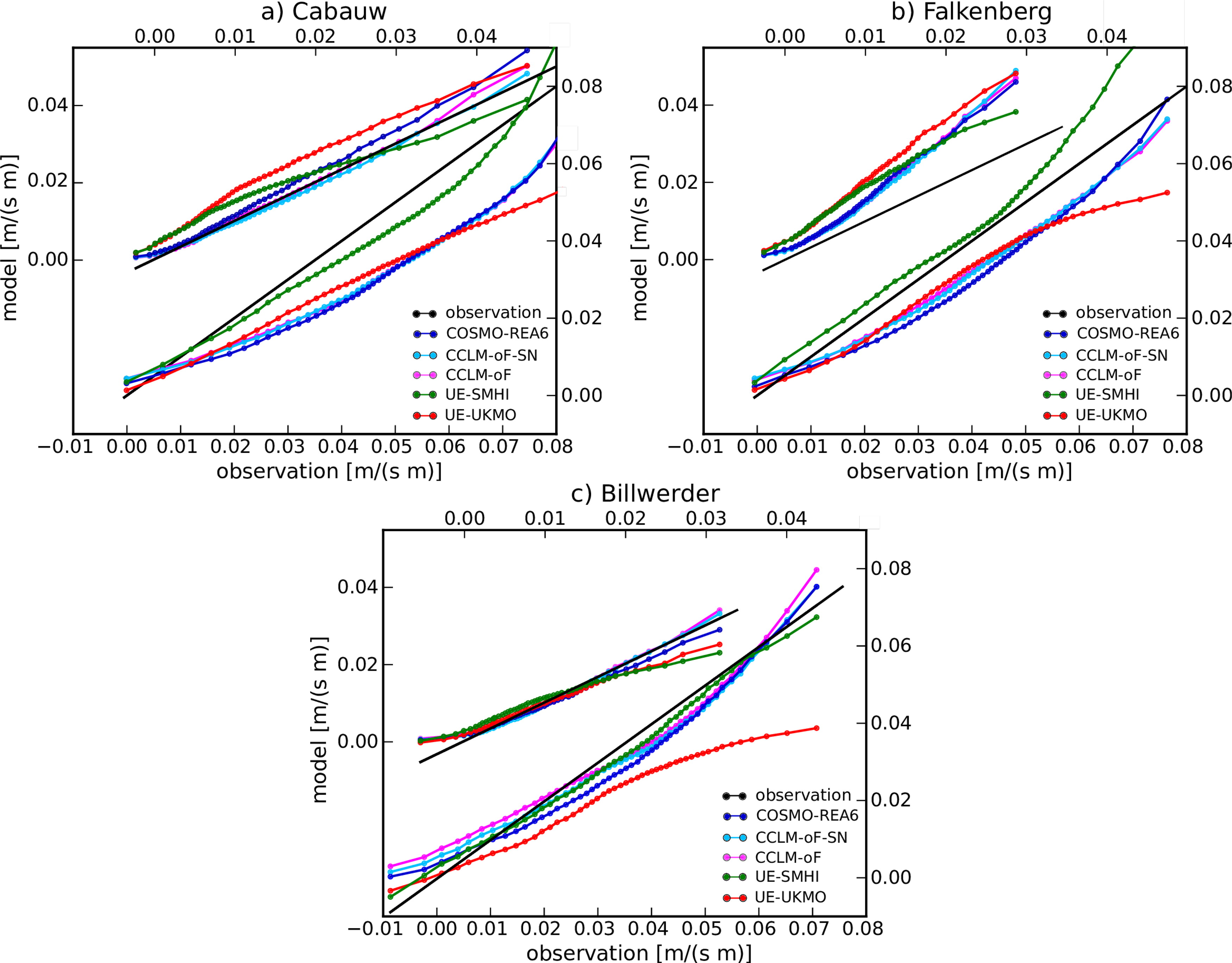
Fig. 9.
Two-year quantile-quantile plot of the vertical gradient in wind speed depending on the stratification at Cabauw (a) (80 m to 20 m), Falkenberg (b) (80 m to 20 m) and Billwerder (c) (110 m to 50 m). Each second quantile (p = 0.02, 0.04, 0.06,…, 0.98, 1.0) of the distribution of simulated gradients is plotted against the quantiles of the observed gradients. The upper part of each figure refers to the unstable stratifications (upper x-axis and left y-axis), and the lower part refers to the very stable stratifications (lower x-axis and right y-axis).
Table 6.
RMSErbc at each tower for hourly data in ‘MJJA’ (summer) and ’NDJFM’ (winter). The heights are grouped for the near-surface, above 100 m and in between.
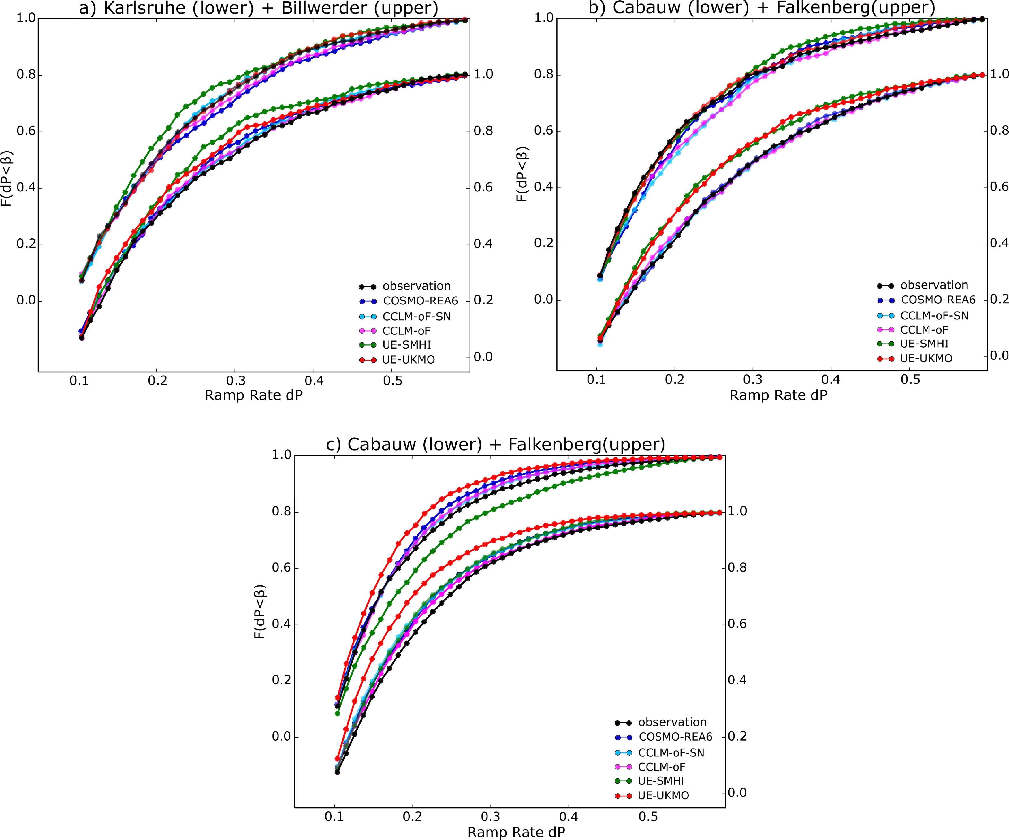
Fig. 10.
Cumulative frequency distribution of 6-hourly ramp events depending on the relative ramp rate for Billwerder at 110 m height and Karlsruhe at 140 m height (a) as well as for Cabauw at 140 m height and Falkenberg at 98 m height (b). (c) is the same as (b) but for 2-hourly ramps.
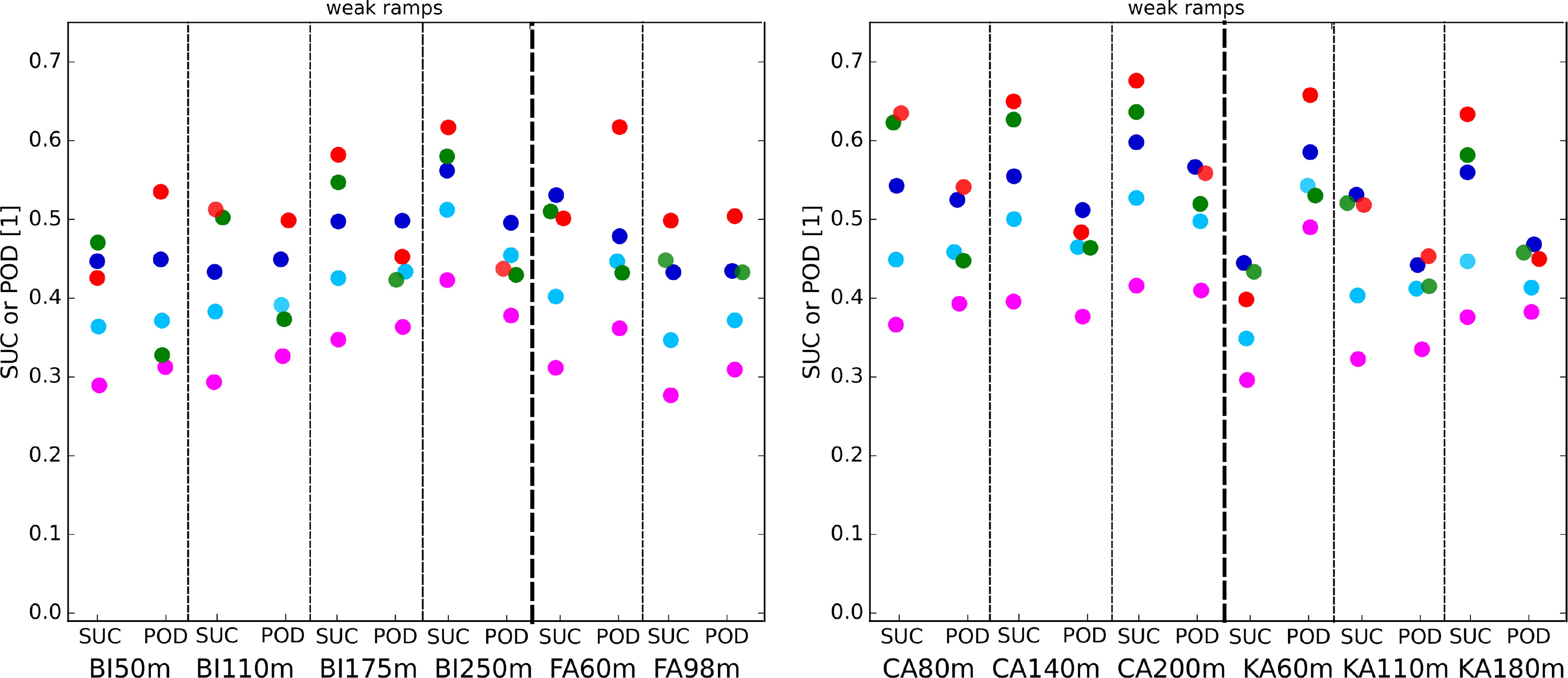
Fig. 11.
Success ratio (SUC) and probability of detection (POD) of ramps for different measurement locations and reanalysis products. The scores are shown for small ramps defined as the percentage change between 15 and 25% and regarding the analysis times 00, 06, 12 and 18 UTC (window length equals 6 hours). The color code is the same as in Figures 9 and 10.