Have a personal or library account? Click to login
A novel generalized combinative procedure for Multi-Scalar standardized drought Indices-The long average weighted joint aggregative criterion Cover

A novel generalized combinative procedure for Multi-Scalar standardized drought Indices-The long average weighted joint aggregative criterion

Open Access
|Jan 2020

Figures & Tables

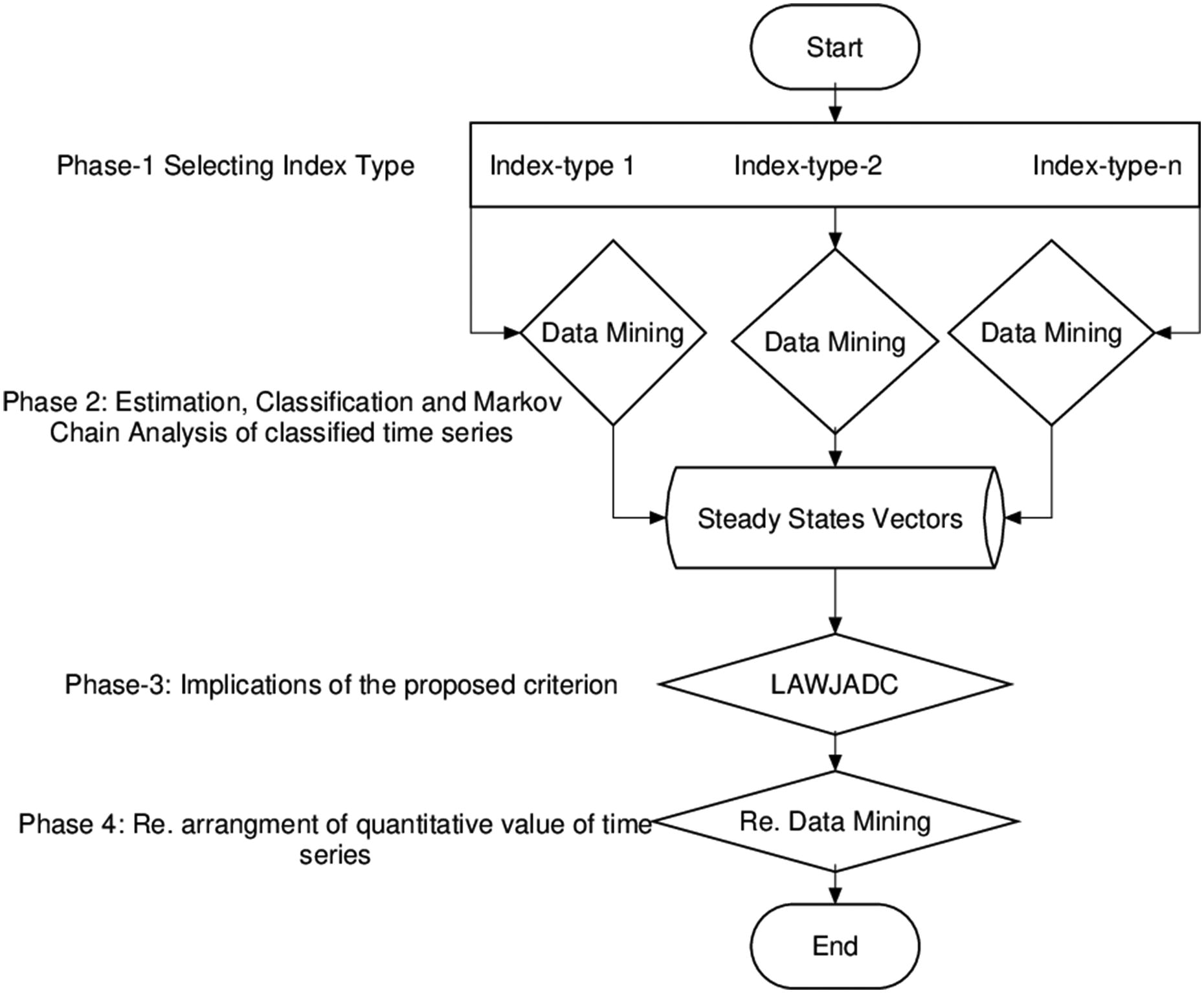
Fig. 1.

Flowchart of the proposed criterion.
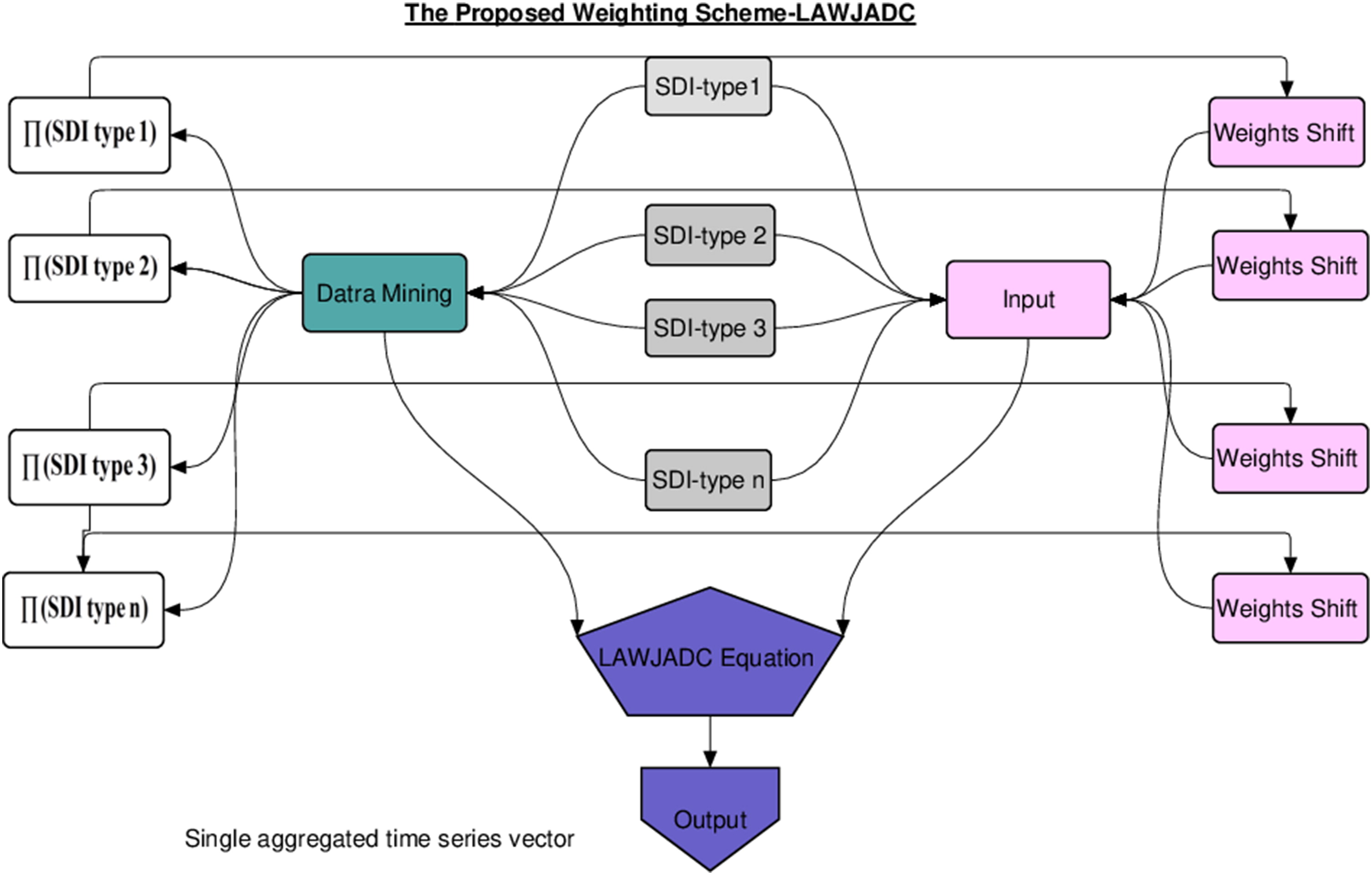
Fig. 2.

Flowchart of the LAWJADC equation.

Table 1.

Drought classification criterion.
Range of Index ValuesClassSDI2Extreme Wet (EW)1.5SDI<2Severe Wet (SW)1SDI<1.5Moderate Wet (MW)1SDI<1Normal Dry (ND) (Near Normal)1>SDI1.5Moderate Dry (MD)1.5>SDI2Severe Dry (SD)SDI<2Extreme Dry (ED)
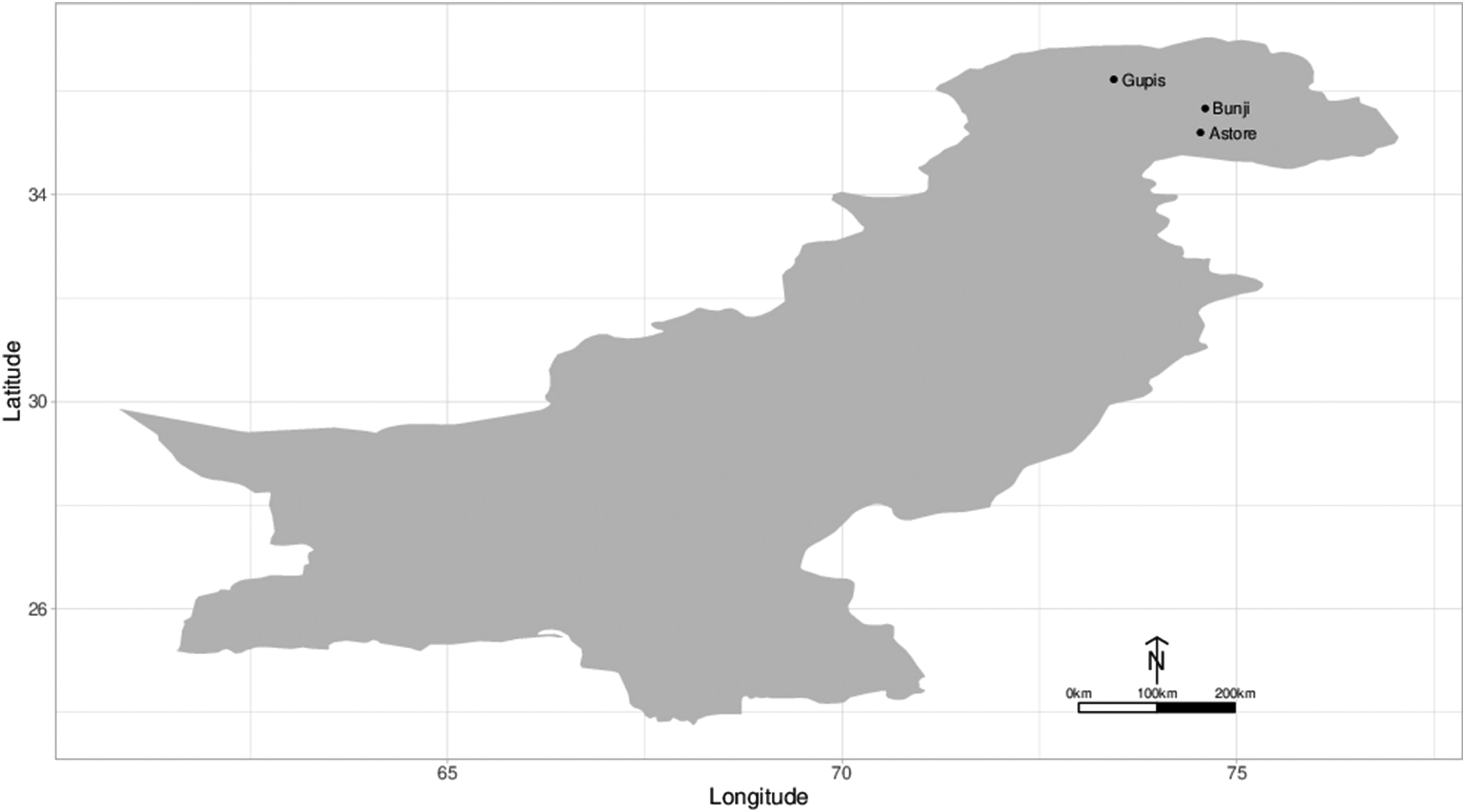
Fig. 3.

Geographical locations of selected meteorological stations of Pakistan.

Table 2.

Climatology of the selected stations.

StationMonthsPrecipitationTemperature (max)Temperature (min)MeanKurtosisMeanKurtosisMeanKurtosisAstore140.0790.9943.033−0.616−7.157−0.165245.5450.7794.4180.805−5.1850.610373.8621.5589.097−0.344−0.8120.106479.4230.64115.4720.2024.083−0.191565.6360.66720.207−0.1727.7840.089624.8−0.77224.647−0.27411.4191.348725.2662.24327.123−0.62514.5050.287825.8380.54426.769−0.44914.4970.204925.55115.81023.251−0.95110.216−0.2711020.9232.65517.8340.7764.6320.8091117.1922.15311.6310.103−0.283−0.5591227.6818.7095.734−0.111−4.397−0.559Bunji16.2334.48110.0410.3000.136−0.60229.5928.26012.776−0.0572.8920.548314.1027.40918.474−0.5457.786−0.674424.9562.34224.467−0.19912.269−0.380527.6791.93628.6970.00615.316−0.152610.60.92633.32−0.31319.21.050717.8753.60035.3860.36622.603−0.210822.4343.23334.91−0.09121.7330.429914.5755.69531.455−0.24516.6741.986107.43624.93525.678−0.09210.592−0.094112.9419.02618.751−0.7114.6962.095124.94512.46712.1790.4271.1560.007Gupis17.4032.3444.681−0.426−5.639−0.561212.13621.0597.0210.577−3.2810.463315.861.75912.625−0.3461.776−0.712440.60611.64119.044−0.5217.104−0.675526.9610.92123.787−0.00810.939−0.180617.8593.84528.8560.06414.9720.024716.0914.37031.705−0.34817.5870.491824.7679.03530.546−0.48016.7630.099913.69813.38126.521−0.11612.4580.040108.0512.39220.555−0.1796.545−0.840112.4831.16614.230.1531.046−0.911124.47510.1816.9320.500−3.454−0.202
Table 3.

BIC for Scale 1 SPI, SPEI and SPTI for Astore Bunji and Gupis.
AstoreBunjiGupisDistributionSPISPEISPTISPISPEISPTISPISPEISPTI2P Beta−735.45−565.00−287.79−722.44−1019.68−125.12−399.44−775.08−254.433P Weibull−1036.51−700.54−483.52−1030.98−1178.06−188.38−777.57−910.74−370.554P Beta−1031.38−700.28−473.37−1020.69−1210.97−181.74−788.69−823.15−374.24Arcsine−853.92−643.79−274.88−791.05−1089.247.71−577.40−817.37−151.87Burr−777.82−656.97−332.22−753.84−1152.29158.50−537.17−905.52−21.11Cauchy−906.22−673.83−357.62−790.41−1147.13−2.03−640.15−884.69−235.77Chi−772.18−571.38−253.75−747.42−1024.70−89.65−535.49−779.77−188.78Chi-Square−778.82−570.07−450.78−771.56−1024.59−49.17−549.29−779.77−146.95Cosine−827.71−706.01−182.80−582.27−1175.57165.44−409.73−880.8013.08Curvilinear Trapezoidal−770.35−590.81−369.28−561.78−1128.83−40.20−399.24−809.67−158.55Exponential−992.52−569.99−398.97−727.50−1024.7030.67−596.82−779.77−206.77F-−735.45−565.75−459.87−863.89−1019.682.54−623.87−775.23−124.81Gamma−1024.97−573.48−482.01−879.99−1019.80−116.91−667.73−775.23−294.28Generalized Extreme Value−959.45−700.89−450.09−886.80−1216.78−88.95−744.99−943.97−338.99Generalized normal−974.59−699.88−472.53−929.73−1208.10−124.81−759.83−938.39−355.54Gumbel−942.14−692.28−382.34−754.06−1159.4529.41−607.56−881.41−205.28Inverse Chi-Square−847.29−573.96−260.44−849.03−1024.7074.59−615.75−779.84−126.69Inverse Gamma−894.39−575.70−393.13−864.79−1019.80−75.36−737.28−775.30−333.93Inverse Gaussian−848.87−565.00−355.22−790.50−1019.68−12.65−740.25−775.08−334.88Johnson SB−971.05−640.08−475.88−925.95−1248.44−122.60−457.52−977.62−351.09Johnson SU−969.88−695.65−467.89−924.84−1203.21−120.21−755.59−936.90−351.09Laplace−914.20−683.10−377.36−756.94−1150.6210.91−630.07−886.00−238.05Logistic−920.09−697.50−356.29−752.10−1166.0937.57−596.22−895.15−187.98Log-normal−970.31−574.42−474.91−882.30−1019.80−105.32−729.92−775.30−338.98Normal−917.65−702.40−348.30−747.38−1170.7946.87−585.58−898.11−172.80Rayleigh−934.02−700.69−365.81−748.60−1166.6042.39−591.38−888.30−182.47Scaled/shifted t-−915.53−698.17−359.42−814.16−1165.90−11.77−642.21−893.57−237.55Skewed-normal−951.45−700.79−378.12−744.10−1218.2744.30−590.96−937.90−185.69Trapezoidal−940.42−710.05−354.12−712.78−1224.0080.19−570.94−946.94−151.71Triangular−945.13−685.96−358.76−664.59−1228.2376.39−557.57−947.69−148.56Uniform−741.92−664.32−220.71−622.63−1084.39121.33−478.66−884.52−37.54von Mises−752.43−568.01−355.83−752.74−1019.8046.82−531.25−775.31−173.35
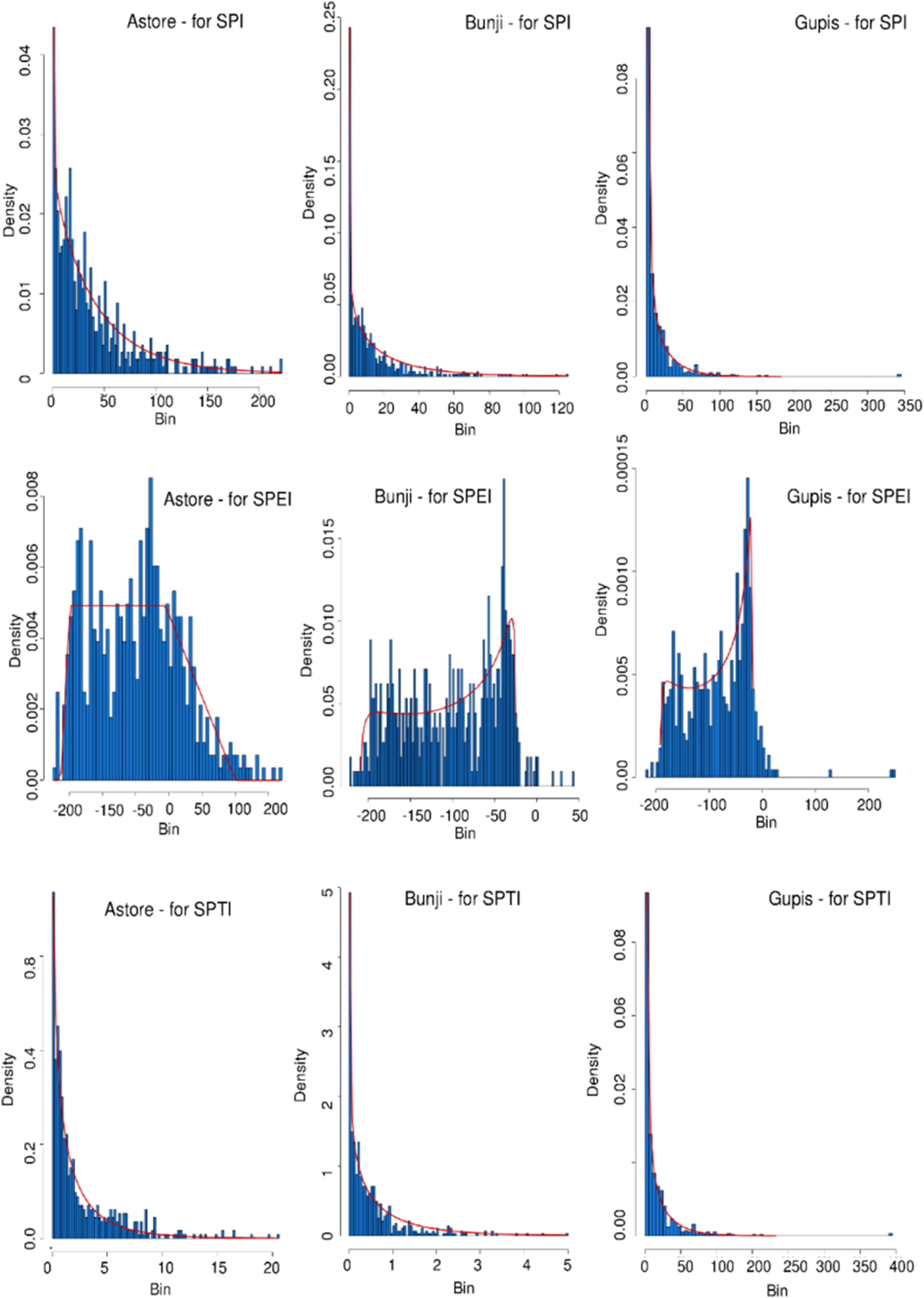
Fig. 4.

Probability distribution at scale one of SPI, SPEI and SPTI at Astore, Bunji and Gupis.

Table 4.

Characteristics of some important distributions.

Sr. NoDistributionsProbability functionCDFRange13P WeibullP(x)=αβxγβα1expxγβαF(x)=1 expxγβαγx<+∞​​2Gammaf(x)=xα1βαΓ(α)expxβF(x)=Γ(α,xβ)Γ(α)x>03Normalf(x)=1σ2πexp12xμσ2F(x)=121+erfxμσ2<x<+4Cosinef(x)=12s1+cosxμsπF(x)=121+xμs+1πsinxμsπμsxμ+s5Skewed normalf(x)=2ω2πexpxξ2ω2αxξω12πexpt22dtF(x)=ϕxξ2ω2Txξ2ω,α
Th,α is Owens Function<x<+6Trapezoidalf(x)=2d+cabxaba for ax<b2d+cab for bx<c2d+cabdxdc for cxdFx=1d+cab1baxa2 for ax<b1d+cab2xab for bx<c11d+cab1dcdx2 for cxdaxd7Triangularf(x)=2xabaca for ax<c2ba for x=c2bxbabc for c<xbF(x)=(xa)²baca for ax<c1(bx)²babc for x=c1 for c<xbaxb8Johnson SUfx=δλ2π z2+1exp12γ+δlnz+z2+12z=xξλFx=ϕγ+δlnz+z2+1ϕ is Laplace integral<x<+9Johnson SBfx=δλ2π z1zexp12γ+δlnz1z2Fx=ϕγ+δlnz1zϕ is Laplace integralξxξ+λ10Log normalf(x)=exp12In(x)μσ2xσ2πfx=12+erfIn(x)μ2σ20<x<+11Laplacefx=12b+expxμbFx=12expxub for xu 112expxub for xuxR12Logisticfx=expxμss1+expxμs2F(x)=11+expxμs<x<+13Gumbelfx=1βexp(z+expz)z=xμβexpexpxμβxR14Rayleighfx=xσ2expx2(2σ2)Fx=1expx22σ20<x<+154P Betaf(x)= (xmin)α1(maxx)β1Bα, β(maxmin)α+β1F(x)= Bxα, βBα, βmin<x<max
Table 5.

BIC for all scale of SPI, SPEI and SPTI indicators at Astore, Bunji and Gupis stations.
AstorBunjiGupisIndexScalesDistributionBICDistributionBICDistributionBICFor SPI13P Weibull−1036.513P Weibull−1030.984P Beta−788.693Gamma−1279.05Gamma−824.87Gamma−1264.956Gamma−892.67Skewed-normal−1162.15Gumbel−1305.359Gamma−896.09Normal−649.05Johnson SU−1518.9612Cosine−913.33Laplace−688.10Johnson SU−937.6124Skewed-normal−1294.42Laplace−843.74Scaled/Shifted t−1407.98For SPEI1Trapezoidal−710.05Johnson SB−1248.44Johnson SB−977.623Trapezoidal−941.49Johnson SB−1323.78Johnson SB−1098.616Trapezoidal−1440.21Johnson SB−1094.44Trapezoidal−1482.599Triangular−1405.81Trapezoidal−976.73Trapezoidal−1513.1212Trapezoidal−1052.48Logistic−1158.15Laplace−1063.6624Johnson SU−1471.48Gumbel−1508.11Laplace−1474.12For SPTI13P Weilbull−483.523P Weibull−188.384P Beta−374.243Johnson SU−542.87Gumbel−190.69Chi-Square−432.186Log-normal−721.00Skewed-normal−300.34Johnson SU−410.049Gamma−725.22Rayleigh−380.83Johnson SU−463.2112Triangular−702.87Laplace−411.86Johnson SU−466.5724Laplace−564.00Trapezoidal−304.73Scaled/Shifted t−629.46
Fig. 5.

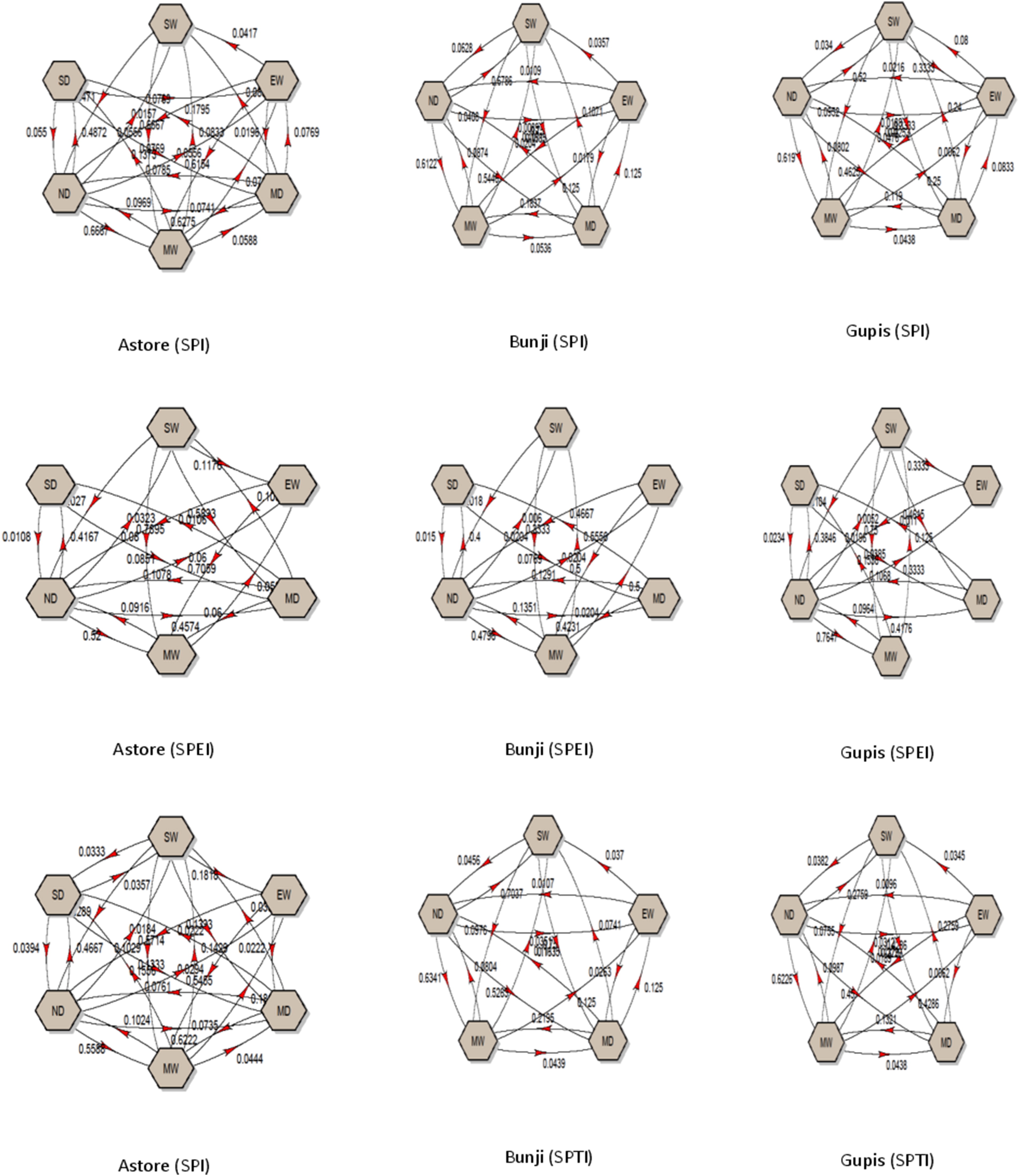
Graphical representation of TPM of SPI, SPEI and SPTI at scale 1 in Astore, Bunji and Gupis.

Table 6.

Steady-states probabilities of various drought classes.
EDEWMDMWNDSDSWSumAstoreSPINA0.023090.092540.095830.676540.069490.042521.0Scale-1SPEINA0.030130.167160.086610.661130.021350.033611.0SPTINA0.019520.079950.118720.678870.053390.049541.0SPINA0.026740.096260.074870.76292NA0.039221.0Scale-3SPEINA0.017560.164750.119970.633950.037610.026161.0SPTINA0.015750.132150.109070.658430.012670.071931.0SPI0.019050.021370.103110.103300.666140.044280.042751.0Scale-6SPEINA0.021510.152330.114700.636200.032260.043011.0SPTINA0.016030.134010.097980.651980.043000.057001.0SPINA0.070270.021620.084680.77117NA0.052251.0Scale-9SPEI0.045730.001780.087880.153500.624730.054240.032131.0SPTI0.007270.017910.106500.085980.678920.049680.053741.0SPI0.011310.019740.106540.111280.667670.056540.026921.0Scale-12SPEI0.024340.023160.094800.098000.685970.057710.016041.0SPTINA0.021360.130680.096100.642460.064910.044491.0SPI0.011110.037040.070370.057410.738890.075930.009261.0Scale-24SPEI0.01667NA0.127780.105560.661110.064810.024071.0SPTINANA0.124070.111110.640740.074070.050001.0SPINA0.021310.284190.074600.57549NA0.044411.0Scale-1SPEINA0.005340.162010.088520.683650.046290.014191.0SPTINA0.012430.284190.094140.55773NA0.051511.0SPI0.012480.010700.055260.076650.778970.016040.049911.0Scale-3SPEINA0.007130.169340.146170.638150.032090.007131.0SPTINA0.026740.096260.074870.76292NA0.039221.0SPINA0.039430.091400.053760.77240NA0.043011.0Scale-6SPEINA0.007130.169340.146170.638150.032090.007131.0SPTINA0.026740.096260.074870.76292NA0.039221.0GupisSPINA0.061260.041440.082880.74955NA0.064861.0Scale-9SPEI0.016220.016220.118920.086490.688290.045050.028831.0SPTINA0.070270.021620.084680.77117NA0.052251.0SPINA0.067030.048910.072460.74457NA0.067031.0Scale-12SPEINA0.036230.103260.105070.695650.005430.054351.0SPTI0.039860.003620.074280.108700.697460.018120.057971.0SPI0.03704NA0.057410.131480.659260.044440.070371.0Scale-24SPEINA0.029630.109260.111110.67037NA0.079631.0SPTINA0.040740.057410.083330.73704NA0.081481.0SPINA0.014220.201210.086950.64801NA0.049611.0Scale-1SPEINA0.007060.185270.171280.593700.026730.015971.0SPTINA0.014240.204720.072750.66037NA0.047931.0SPINA0.026740.096260.074870.76292NA0.039221.0Scale-3SPEINA0.017560.164750.119970.633950.037610.026161.0SPTINA0.015750.132150.109070.658430.012670.071931.0SPI0.019050.021370.103110.103300.666140.044280.042751.0Scale-6SPEINA0.021510.152330.114700.636200.032260.043011.0SPTINA0.016030.134010.097980.651980.043000.057001.0BunjiSPINA0.070270.021620.084680.77117NA0.052251.0Scale-9SPEI0.045730.001780.087880.153500.624730.054240.032131.0SPTI0.007270.017910.106500.085980.678920.049680.053741.0SPI0.011310.019740.106540.111280.667670.056540.026921.0Scale-12SPEI0.024340.023160.094800.098000.685970.057710.016041.0SPTINA0.021360.130680.096100.642460.064910.044491.0SPINANA0.148150.127780.611110.048150.064811.0Scale-24SPEI0.05185NA0.061110.187040.646300.048150.005560.9SPTINANA0.144440.135190.611110.027780.081481.0
Fig. 6.

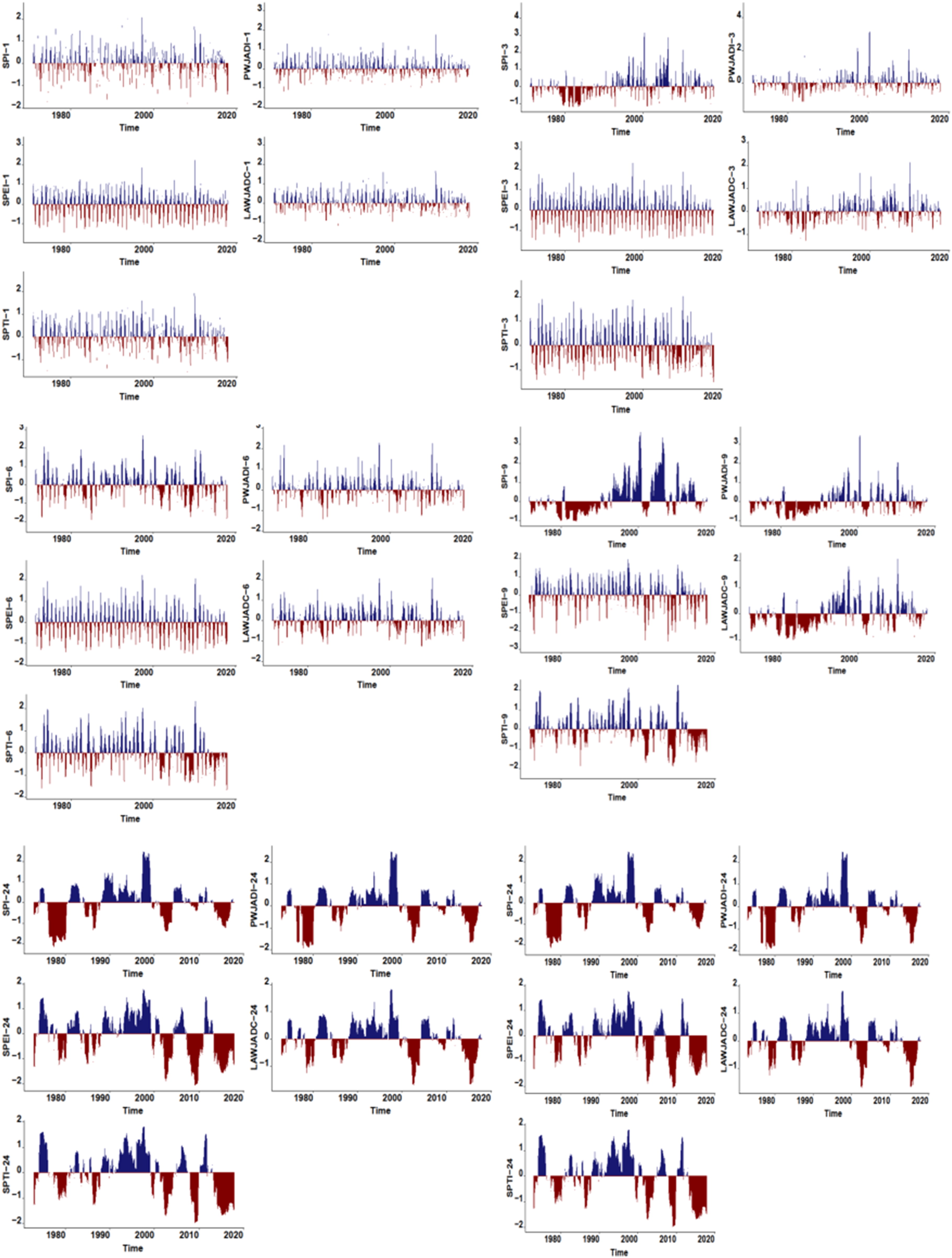
Temporal plot of SPI, SPEI, SPTI, PWJADI and LAWJADC for Astore.
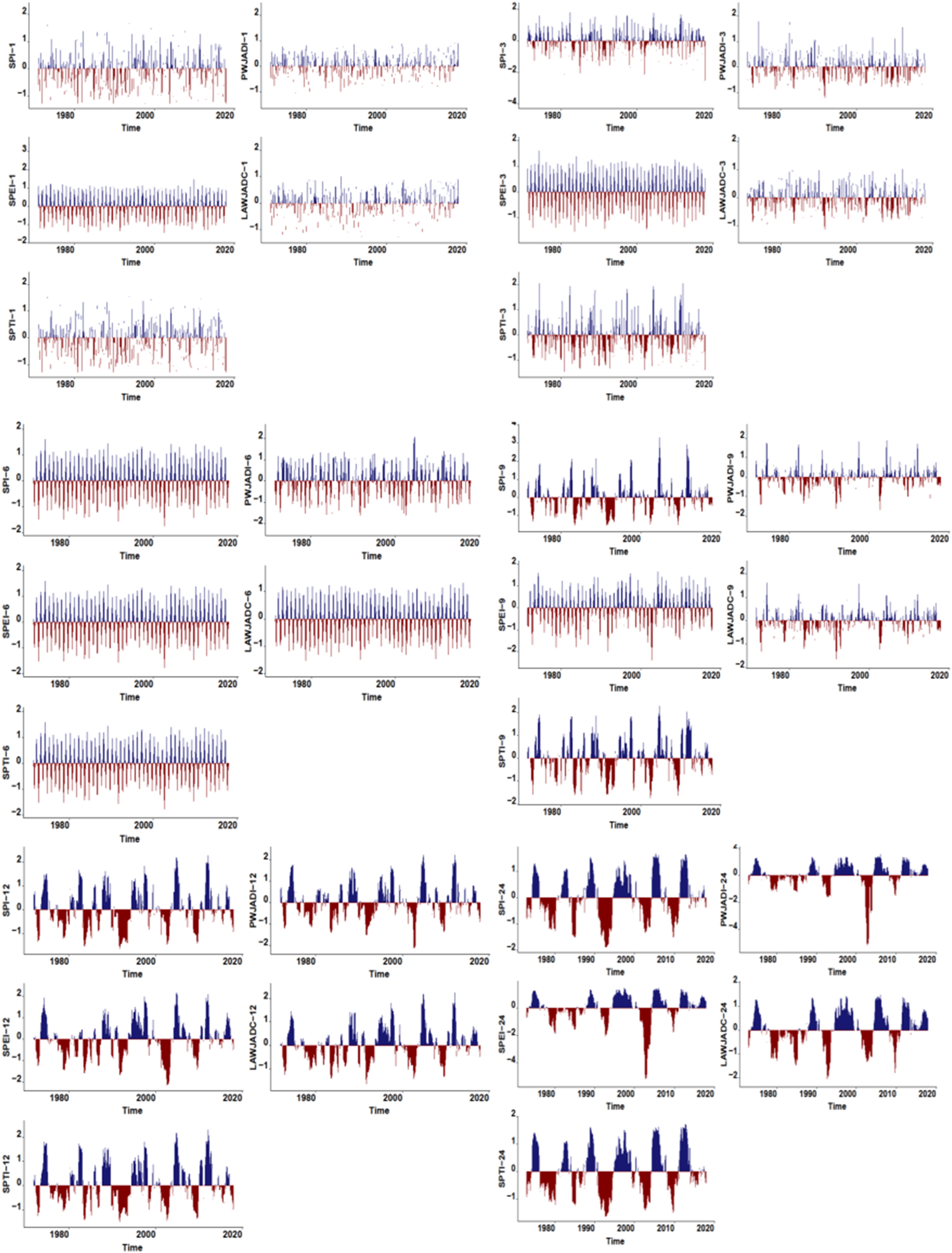
Fig. 7.

Temporal plot of SPI, SPEI, SPTI, PWJADI and LAWJADC for Bunji.
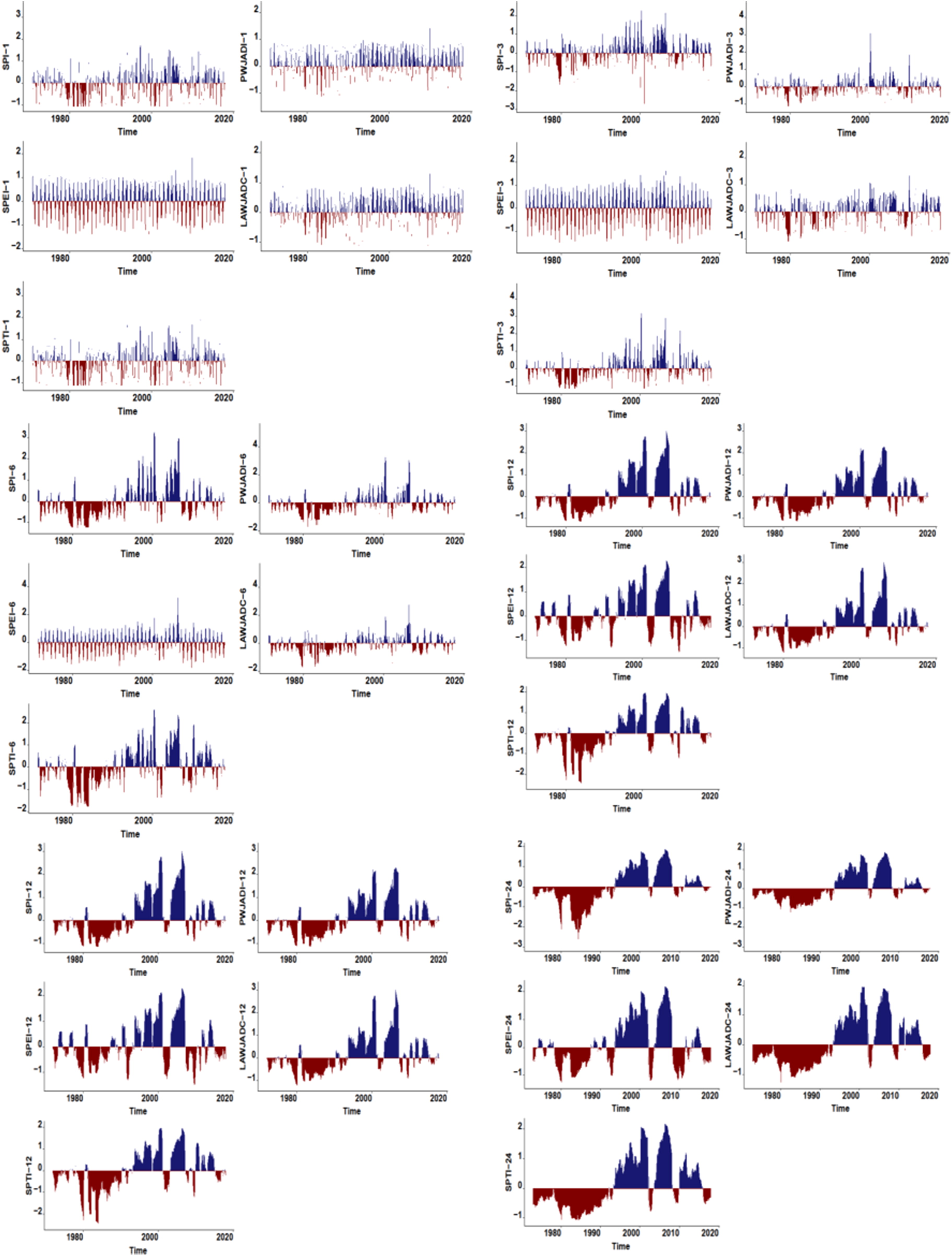
Fig. 8.

Temporal plot of SPI, SPEI, SPTI, PWJADI and LAWJADC for Gupis.
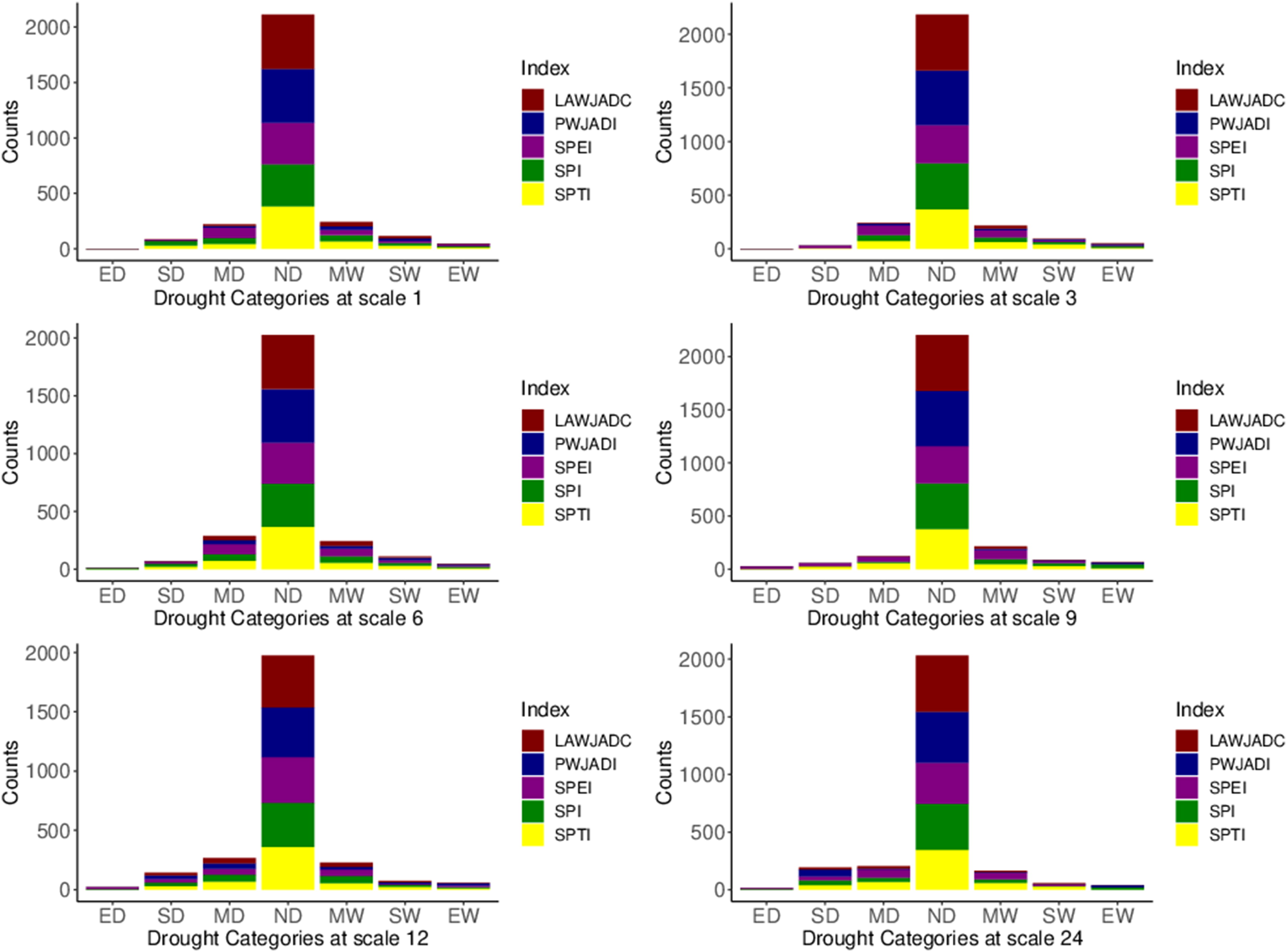
Fig. 9.

Bar plot counts of drought categories observed in SPI, SPEI, SPTI, PWJADI and LAWJADC for Astore.
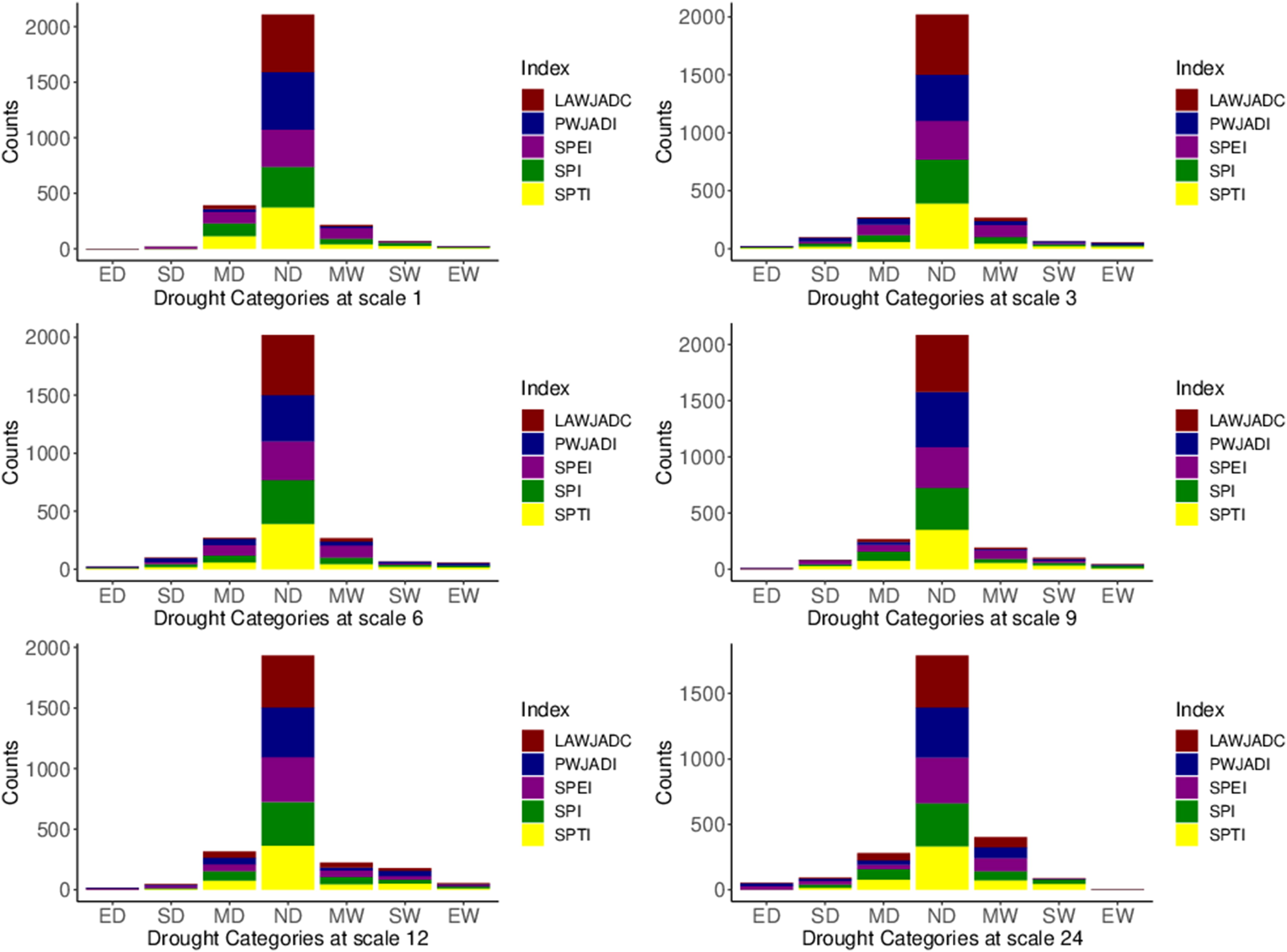
Fig. 10.

Bar plot counts of drought categories observed in SPI, SPEI, SPTI, PWJADI and LAWJADC for Bunji.
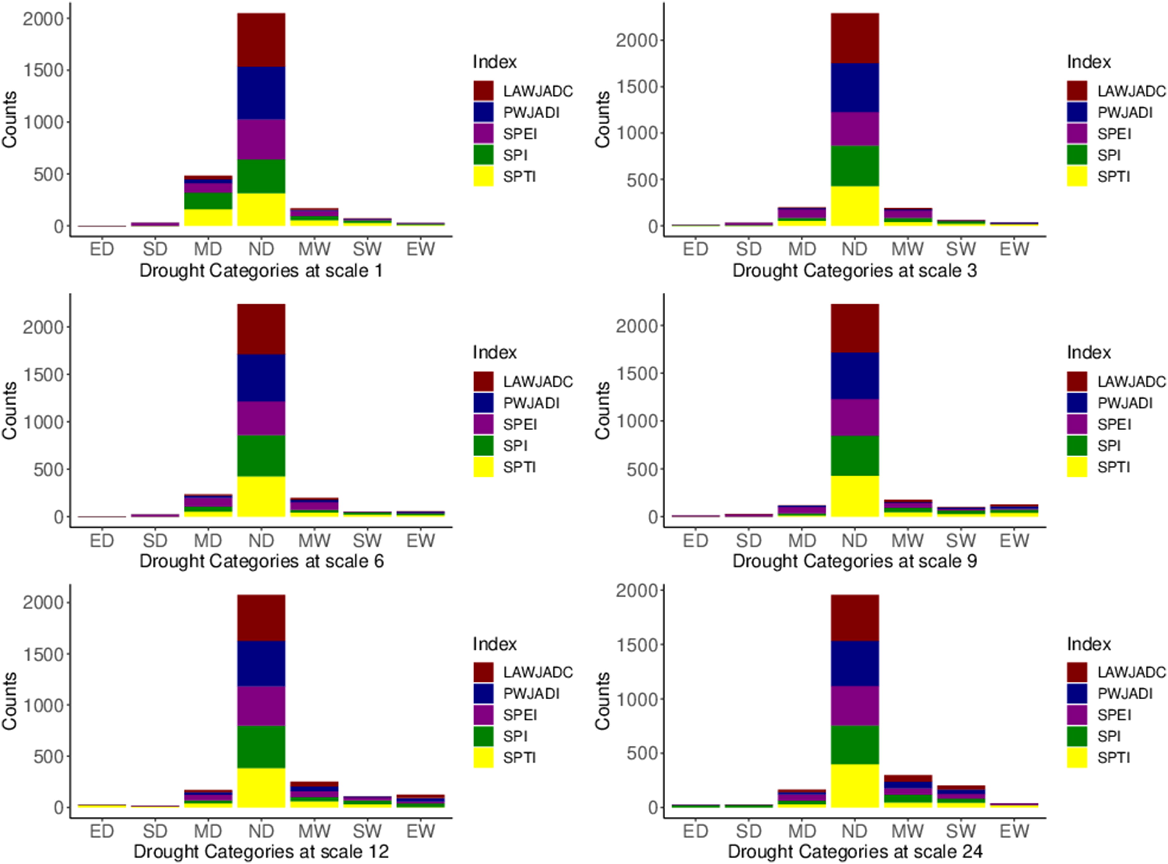
Fig. 11.

Bar plot counts of drought categories observed in SPI, SPEI, SPTI, PWJADI and LAWJADC for Gupis.

Table 7.

Kappa values showing association among various drought indices and criterion.

KappaP-valueStationScaleMethodSPISPEISPTIPWJADILAWJADCSPISPEISPTIPWJADILAWJADCScale-1LAWJADC0.28500.01760.22200.82501.00000.00000.60300.00000.00000.0000AstorePWJADI0.29700.09700.24301.00000.82500.00000.00480.00000.00000.0000Scale-3LAWJADC0.26500.10600.10900.48001.00000.00000.00020.00020.00000.0000PWJADI0.48400.03810.16301.00000.48000.00000.29200.00000.00000.0000Scale-6LAWJADC0.39000.17300.27900.55601.00000.00000.00000.00000.00000.0000PWJADI0.32100.40600.38701.00000.55600.00000.00000.00000.00000.0000Scale-9LAWJADC0.21800.02630.06150.63201.00000.00000.25800.02160.00000.0000PWJADI0.43200.01890.15901.00000.63200.00000.55700.00000.00000.0000Scale-12LAWJADC0.18500.00290.49600.39201.00000.00000.94000.00000.00000.0000PWJADI0.29600.36300.53101.00000.39200.00000.00000.00000.00000.0000Scale-24LAWJADC0.17300.32500.31400.06831.00000.00000.00000.00000.08800.0000PWJADI0.45000.06380.05151.0000−0.06830.00000.07170.21000.00000.0880Scale-1LAWJADC0.34300.11900.28500.90401.00000.00000.00020.00000.00000.0000BunjiPWJADI0.29800.17100.29901.00000.90400.00000.00000.00000.00000.0000Scale-3LAWJADC0.11600.06890.23300.61601.00000.00000.00470.00000.00000.0000PWJADI0.15300.15300.36401.00000.61600.00000.00000.00000.00000.0000Scale-6LAWJADC0.07270.13000.18400.17301.00000.00640.00000.00000.00000.0000PWJADI0.59900.03630.62701.00000.17300.00000.38200.00000.00000.0000Scale-9LAWJADC0.22400.20600.26700.57801.00000.00000.00000.00000.00000.0000PWJADI0.29300.25400.29501.00000.57800.00000.00000.00000.00000.0000Scale-12LAWJADC0.48900.50800.56700.67501.00000.00000.00000.00000.00000.0000PWJADI0.53800.56800.75601.00000.67500.00000.00000.00000.00000.0000Scale-24LAWJADC0.22000.60100.27700.73001.00000.00000.00000.00000.00000.0000PWJADI0.39200.55200.40701.00000.73000.00000.00000.00000.00000.0000Scale-1LAWJADC0.20600.12800.22500.91201.00000.00000.00040.00000.00000.0000GupisPWJADI0.21200.18300.24501.00000.91200.00000.00000.00000.00000.0000Scale-3LAWJADC0.1420−0.01090.20400.65901.00000.00000.66800.00000.00000.0000PWJADI0.20000.01450.40101.00000.65900.00000.65300.00000.00000.0000Scale-6LAWJADC0.33400.05810.28800.65601.00000.00000.04780.00000.00000.0000PWJADI0.55000.07390.07391.00000.65600.00000.04610.04610.00000.0000Scale-9LAWJADC0.40200.13900.49600.58501.00000.00000.00010.00000.00000.0000PWJADI0.60300.14900.73401.00000.58500.00000.00020.00000.00000.0000Scale-12LAWJADC0.75200.30600.07150.87801.00000.00000.00000.07820.00000.0000PWJADI0.71000.37900.02641.00000.87800.00000.00000.52000.00000.0000Scale-24LAWJADC0.58600.17500.08090.87701.00000.00000.00000.04000.00000.0000Scale-24PWJADI0.54300.19300.06581.00000.87700.00000.00000.11400.00000.0000
Language: English
Page range: 1736248 - 1736248
Published on: Jan 1, 2020
Published by: Stockholm University Press
In partnership with: Paradigm Publishing Services

© 2020 Zulfiqar Ali, Ibrahim M. Almanjahie, Ijaz Hussain, Muhammad Ismail, Muhammad Faisal, published by Stockholm University Press
This work is licensed under the Creative Commons Attribution 4.0 License.