
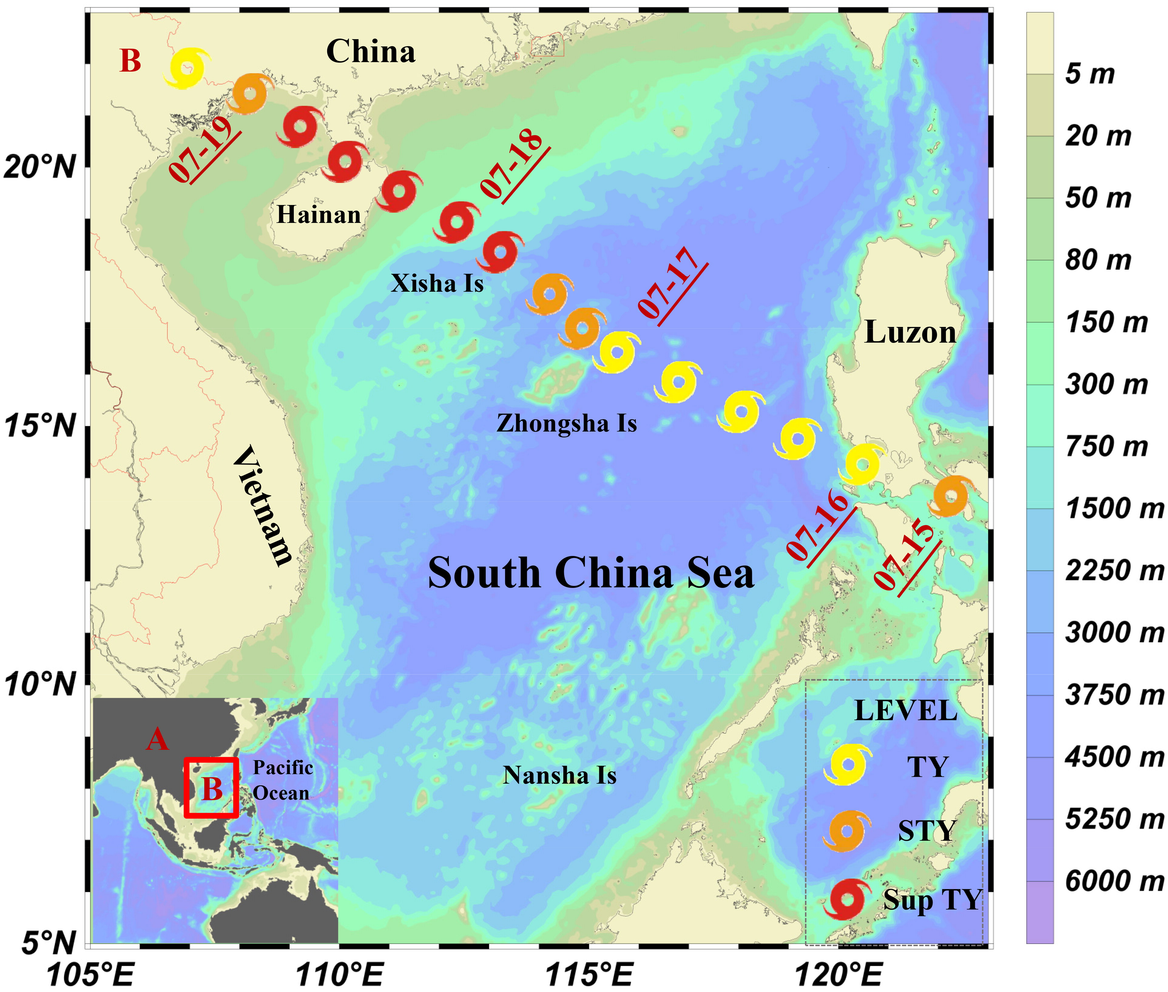
Fig. 1.
The depth of the South China Sea and the best track of super typhoon Rammasun in 2014.
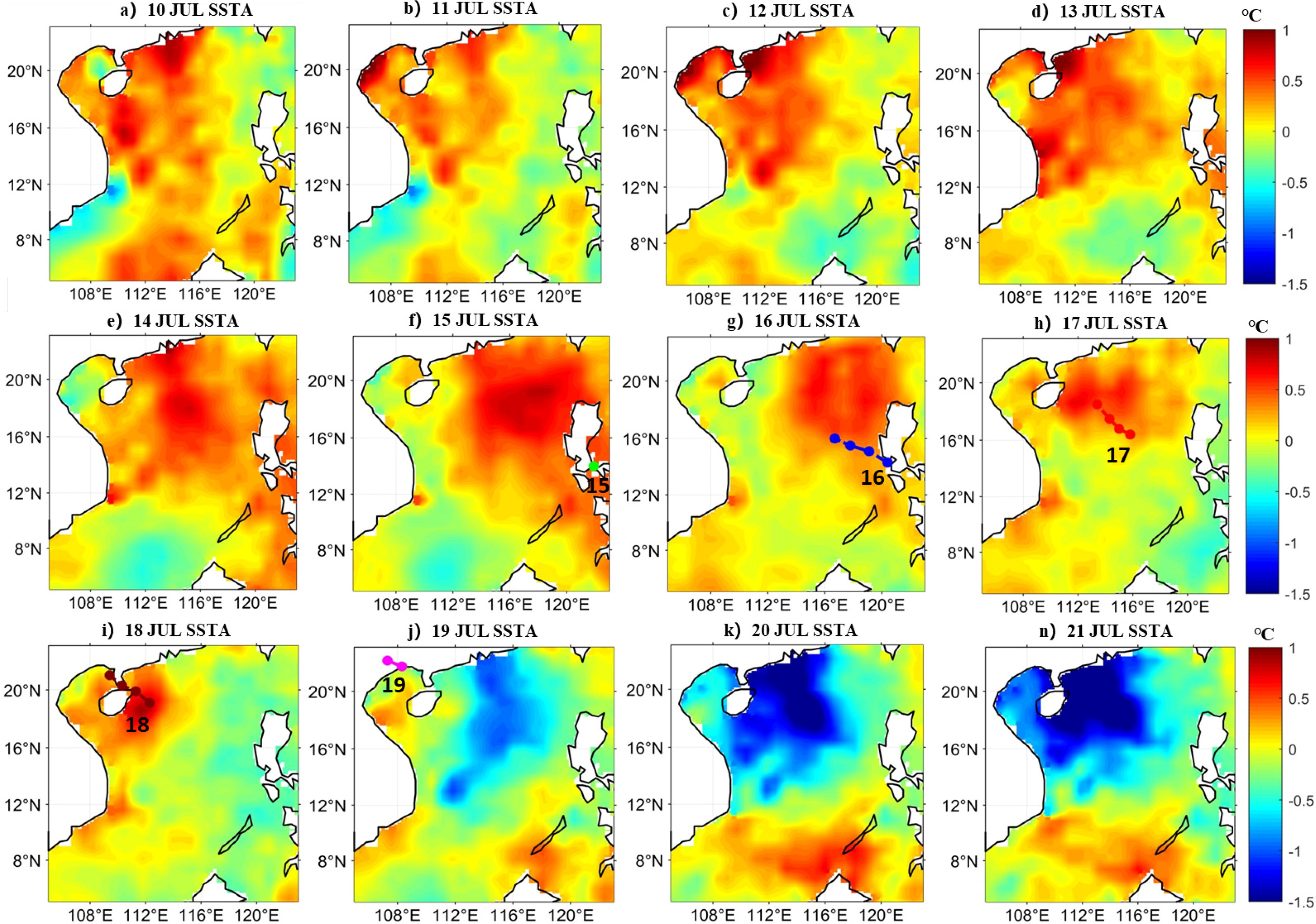
Fig. 2.
Values of SSTA (°C) before (10-a, 11-b, 12-c, 13-d, 14-e, 15-f day), during (16-g, 17-h, 18-i, 19-j day) and after (20-k, 21-n day) the typhoon from July 10 to 21, 2014.
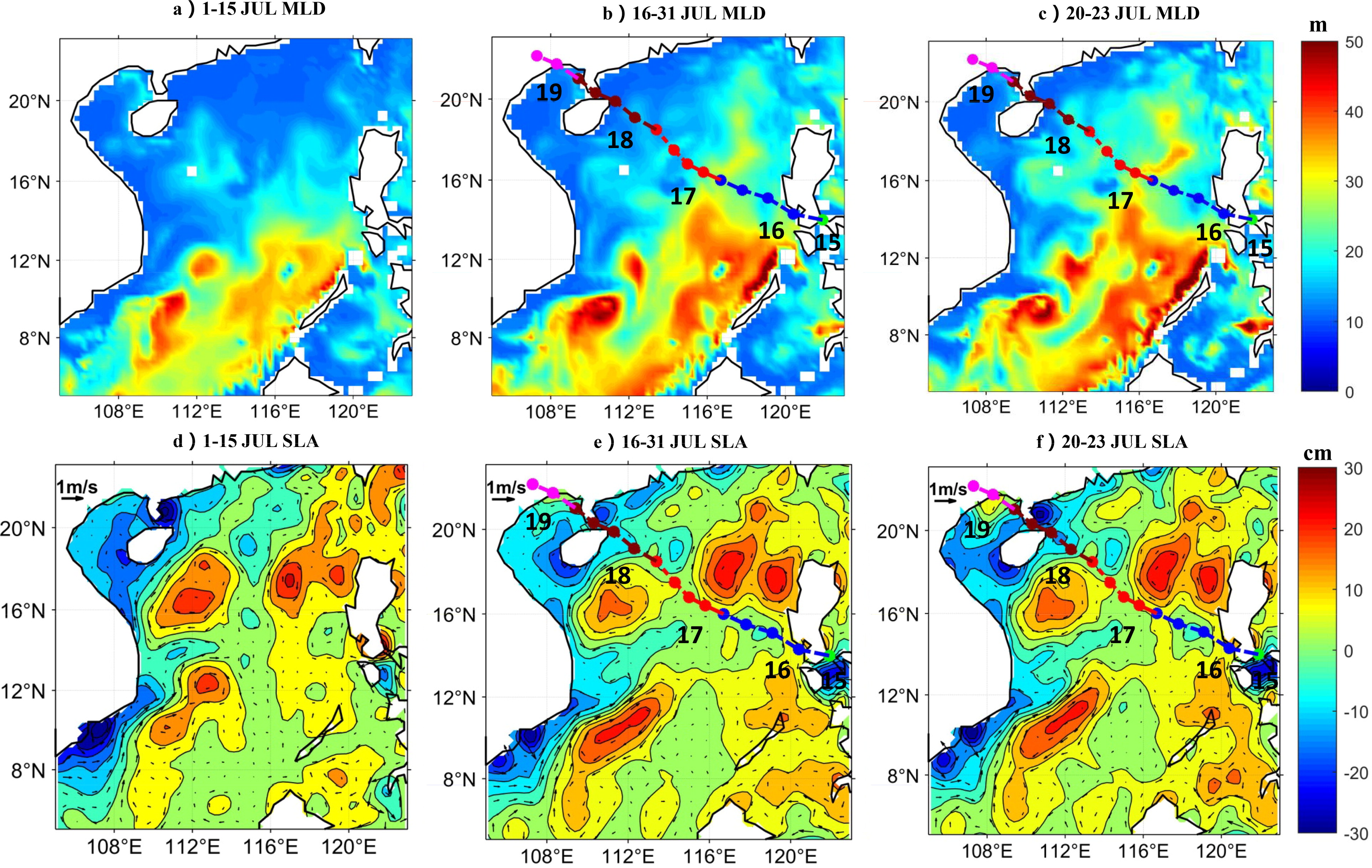
Fig. 3.
The mean fields for sea surface MLD and SLA. (a) MLD (m), 1–15 July. (b) MLD (m), 16–31 July. (c) MLD (m), 20–23 July. (d) SLA (cm), 1–15 July. (e) SLA (cm), 16–31 July. (f) SLA (cm), 20–23 July. Contour intervals of the subfigures in the bottom row are 10 cm.
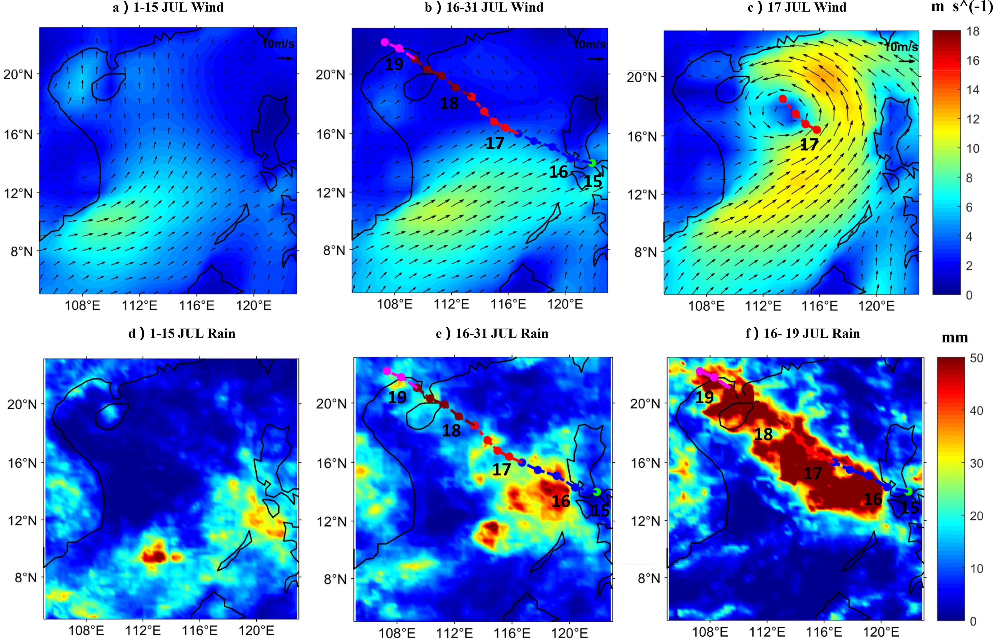
Fig. 4.
The mean fields for SSW and precipitation. (a) SSW (m s-1), 1–15 July. (b) SSW (m s-1), 16–31 July. (c) SSW (m s-1), 17 July. (d) Precipitation (mm), 1–15 July. (e) Precipitation (mm), 16–31 July. (f) Precipitation (mm), 16–19 July.
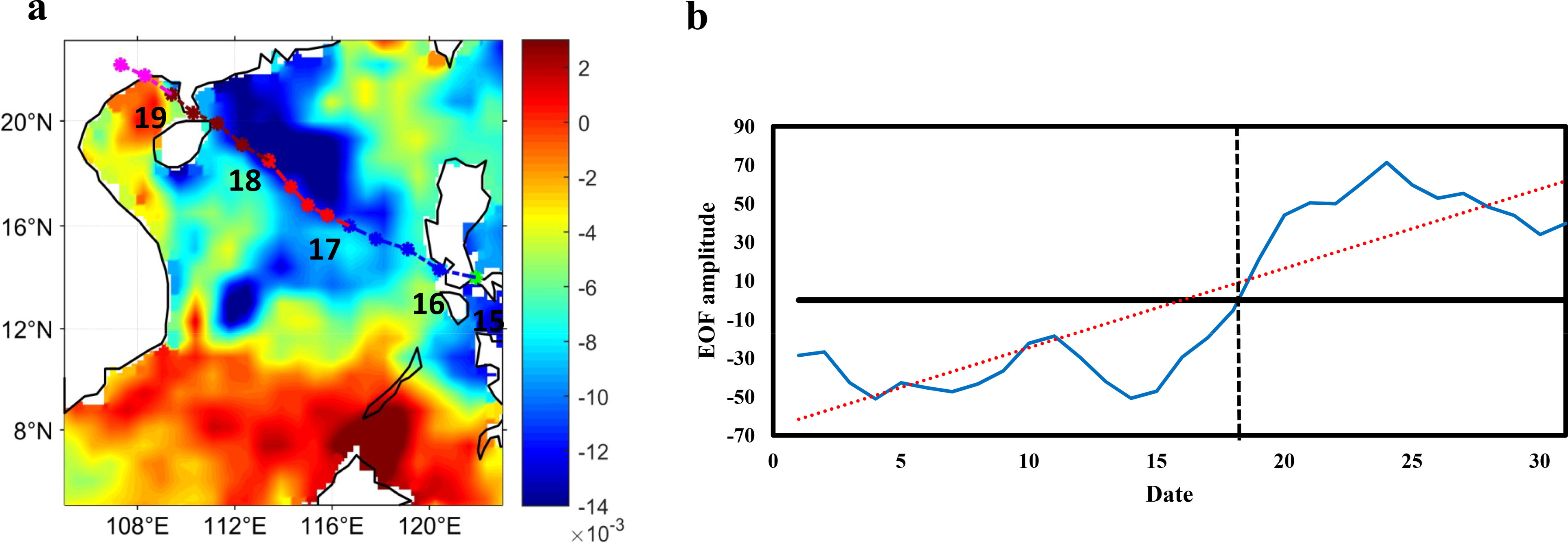
Fig. 5.
The spatial mode (a) and temporal mode (b) of the first diurnal empirical orthogonal function of the sea surface temperature from 1–31 July 2014.
Table 1.
Contributions (1–4) of diurnal empirical orthogonal function modes to SST, SLA, MLD, SSW and precipitation, the fifth column indicates the residual (Res) from the first four modes.
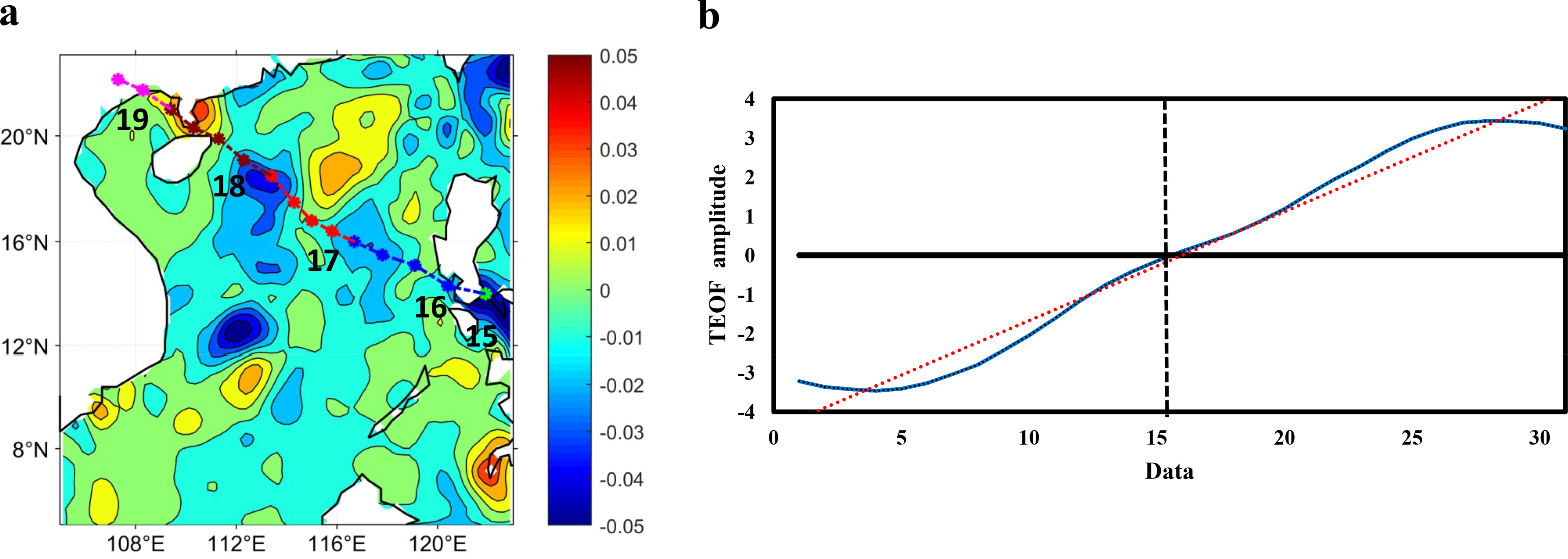
Fig. 6.
The spatial mode (a) and the temporal mode (b) of the first diurnal empirical orthogonal function of the surface level anomaly from 1–31 July 2014.
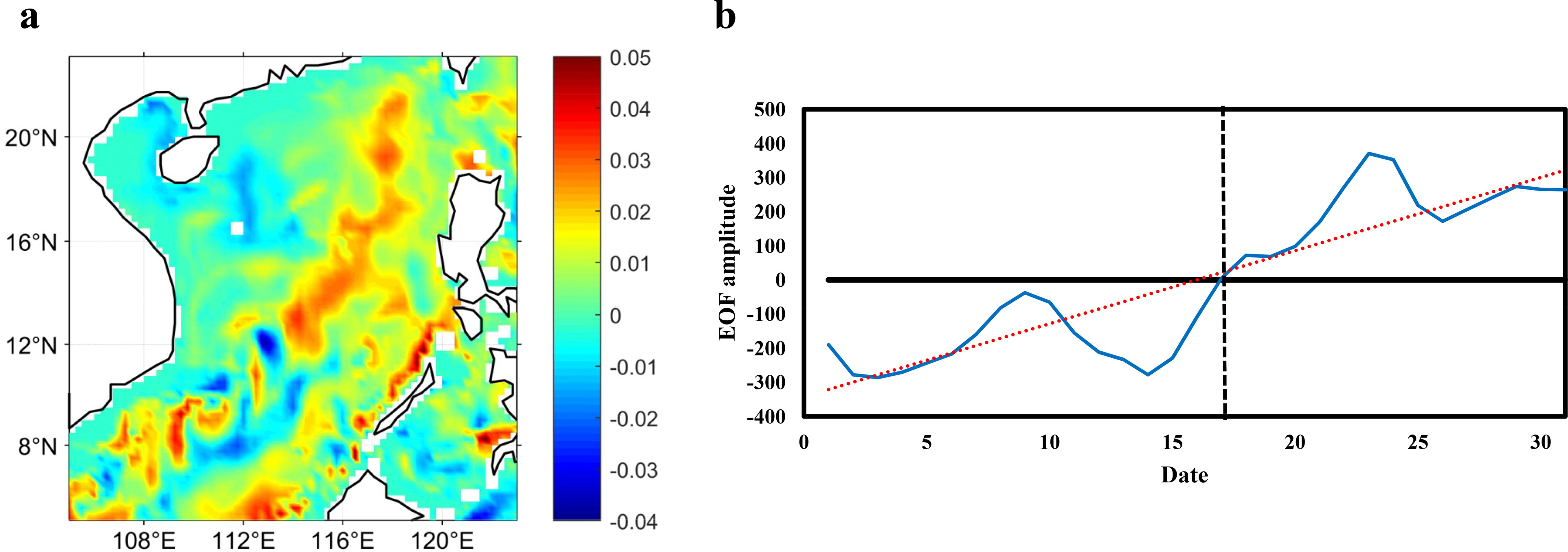
Fig. 7.
The spatial mode (a) and temporal mode (b) of the first diurnal empirical orthogonal function of the mixed layer depth from 1–31 July 2014.
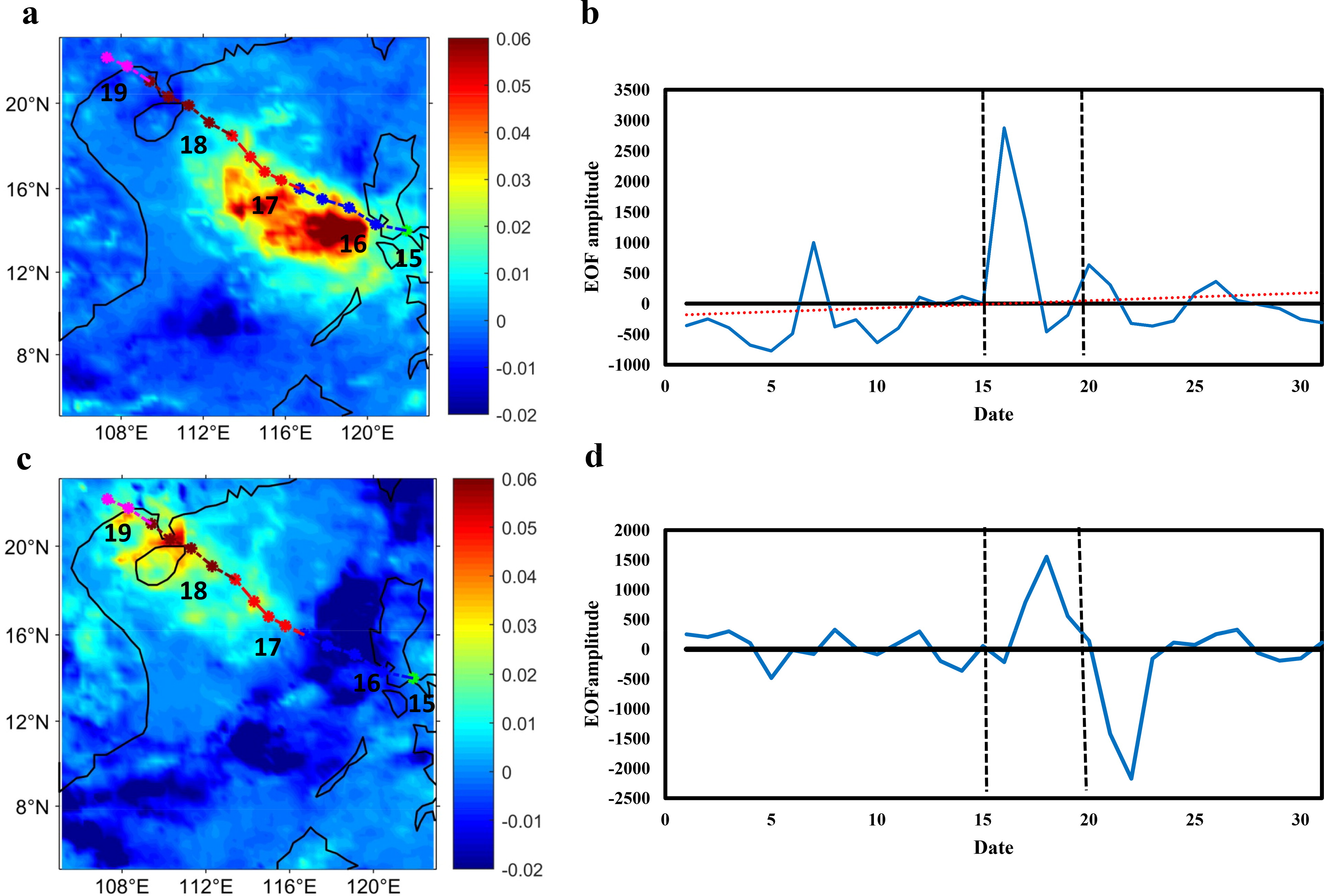
Fig. 8.
The spatial modes (a and c) and temporal modes (b and d) of the first (a and b) and second (c and d) diurnal empirical orthogonal function of precipitation from 1–31 July 2014.
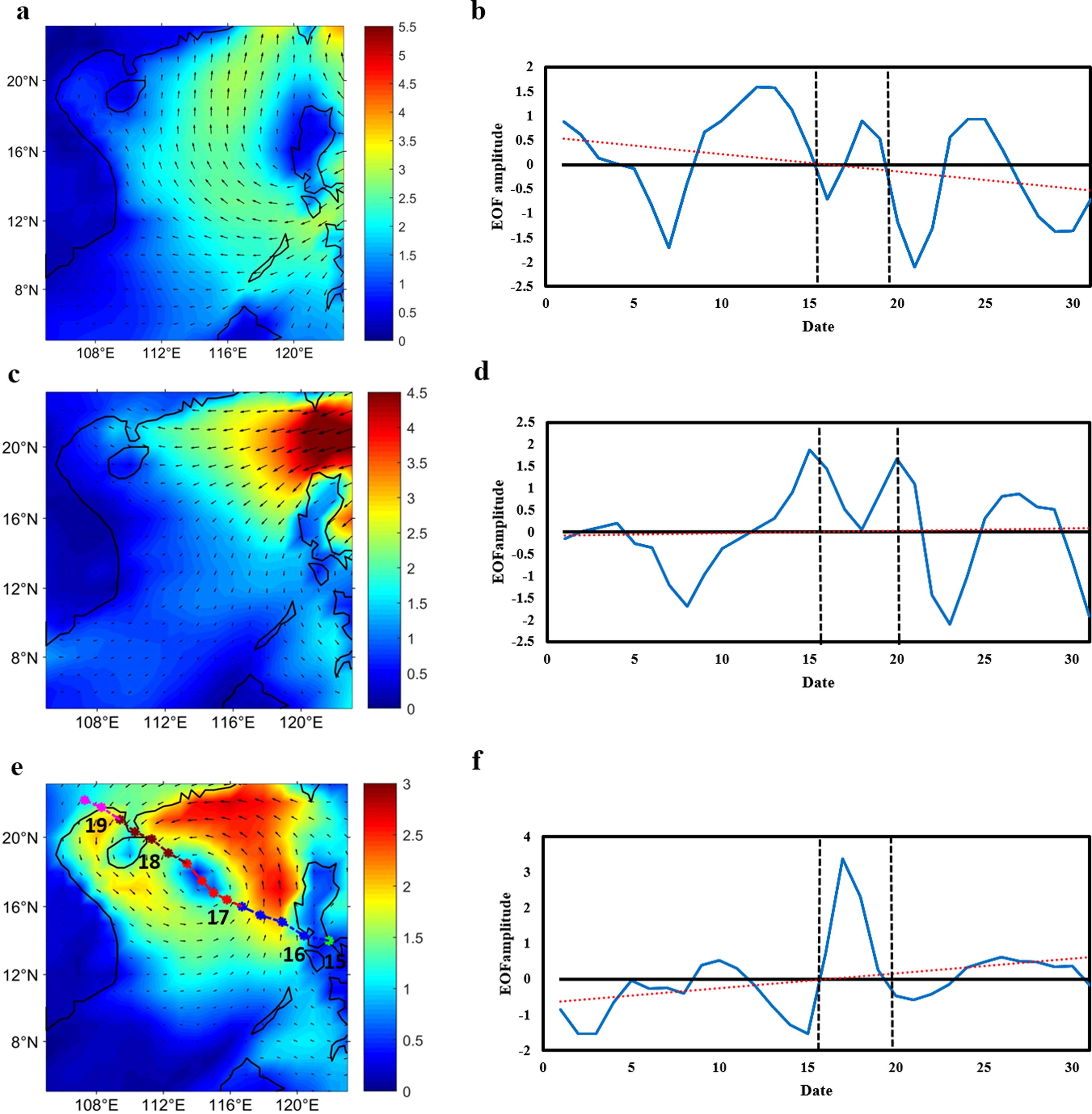
Fig. 9.
The spatial mode (a, c and e) and temporal mode (b, d and f) of the first (a and b), second (c and d) and third (e and f) diurnal empirical orthogonal function modes of sea surface wind from 1–31 July 2014.
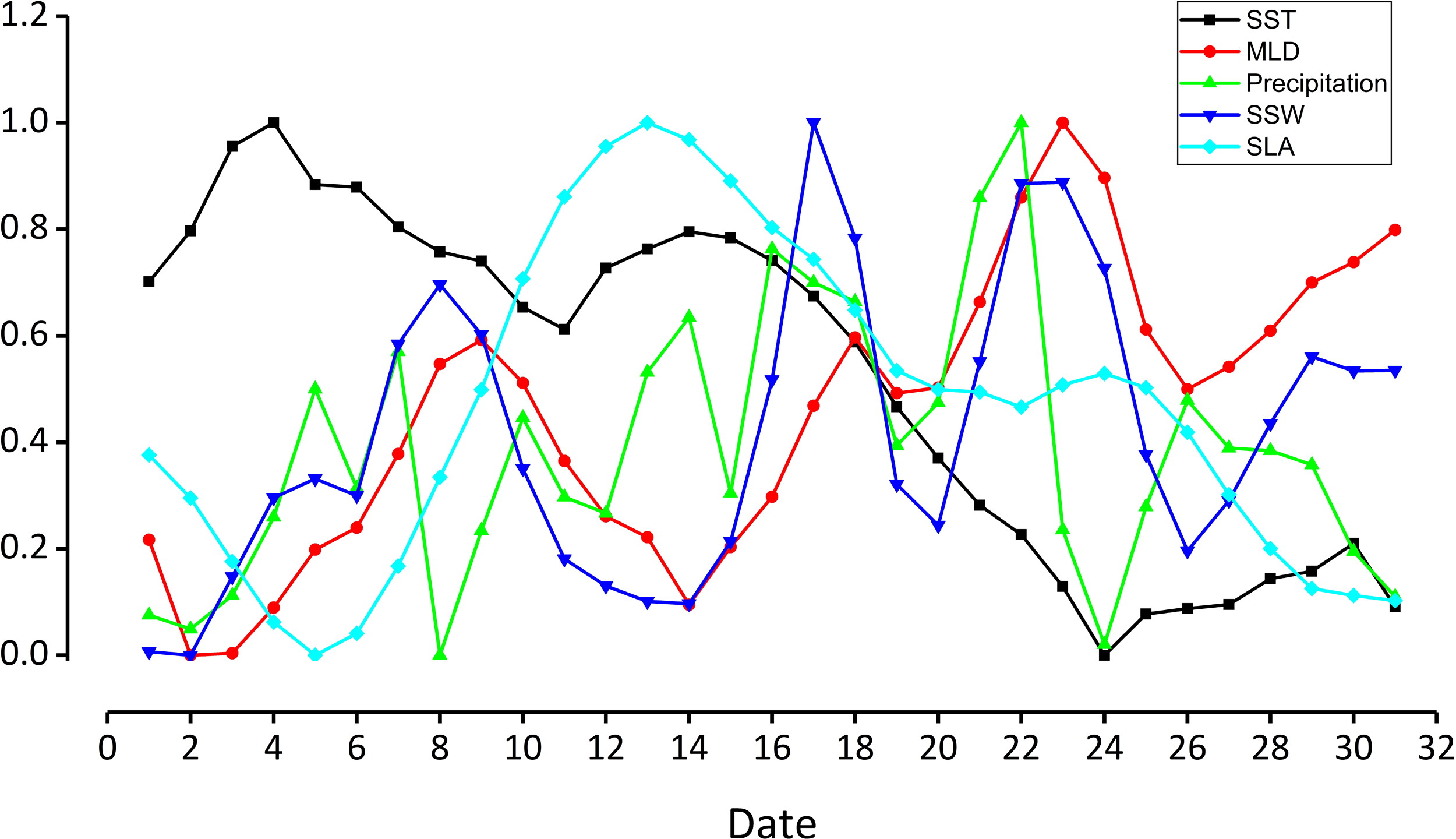
Fig. 10.
Normalized average variation of SST, MLD, SLA, SSW and precipitation of the South China Sea (105°–123°E, 5°–23°N) in July 2014.
Table 2.
Correlation analysis of the average variation of SST, MLD, SSW, SLA and precipitation of the South China Sea.
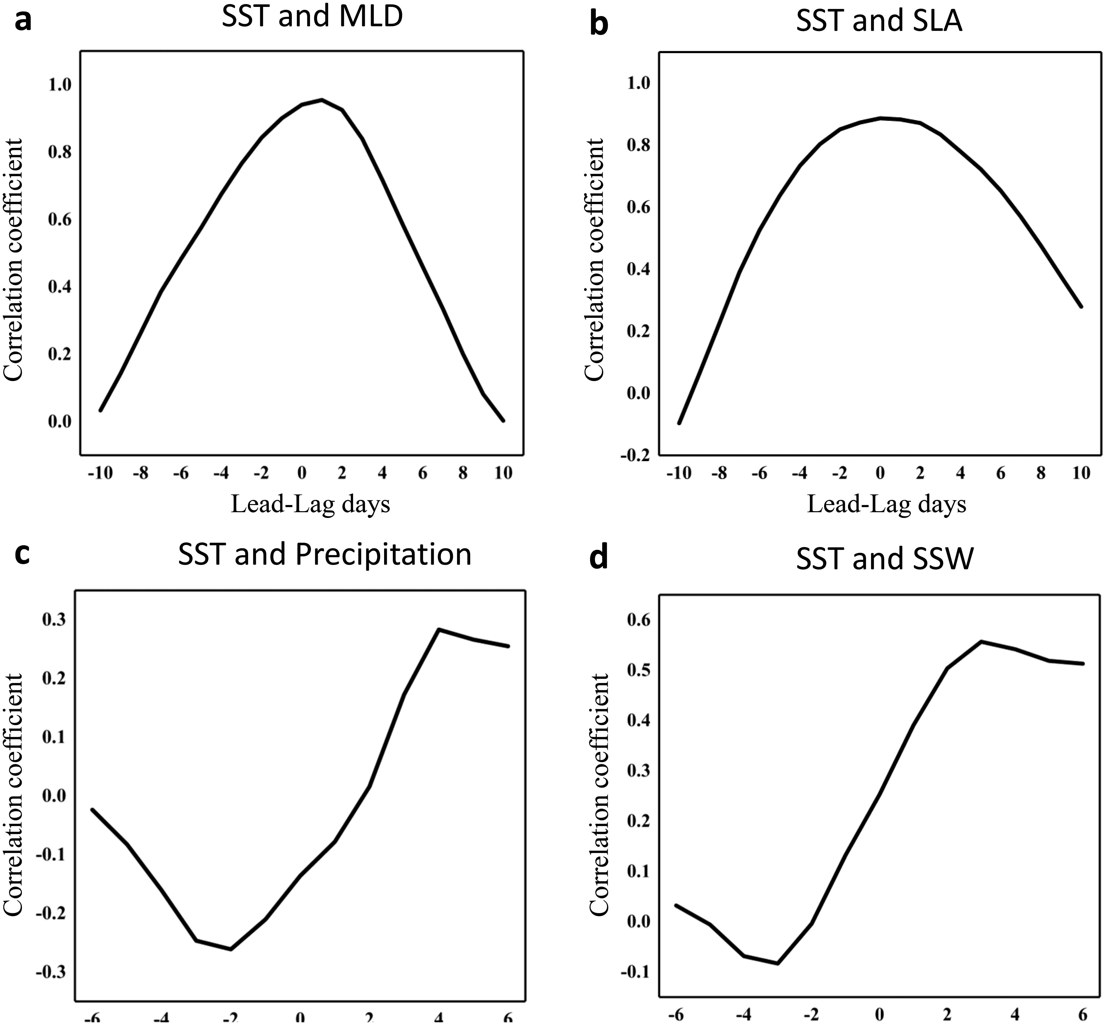
Fig. 11.
The correlations of the time coefficient functions for different lag days. (a) Time coefficient functions of the EOF-1 modes of SST and MLD. (b) Time coefficient functions of the EOF-1 modes of SST and surface level anomaly (SLA). (c) Time coefficient functions of the EOF-1 mode of SST and the mean of the EOF-1 and EOF-2 modes of precipitation. (d) Time coefficient functions of the EOF-1 mode of SST and the EOF-3 mode of SSW.