
Table 1.
List of mathematical symbols.
Table 2.
Temperature tendencies in OpenIFS model.
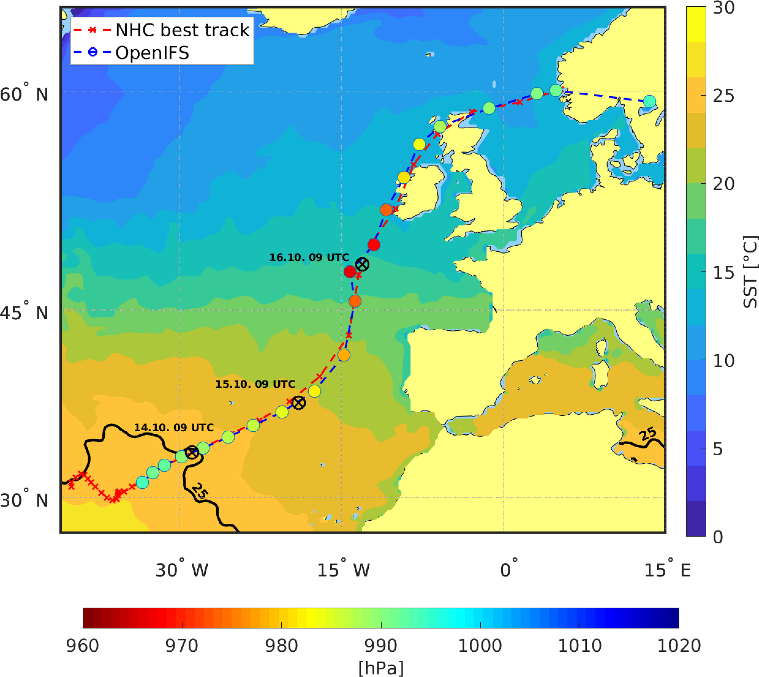
Fig. 1.
National Hurricane Center best track for Hurricane Ophelia (red) and OpenIFS track based on minimum sea level pressure (blue). The colours in the OpenIFS track denote minimum sea level pressure in the OpenIFS simulation. The background colours show the sea surface temperatures at 12 UTC 14 October, with 25 °C isotherm contoured. The locations of Ophelia at its peak intensity as a hurricane (9 UTC 14 October), and 24 (9 UTC 15 October) and 48 hours later (9 UTC 16 October) are also indicated.
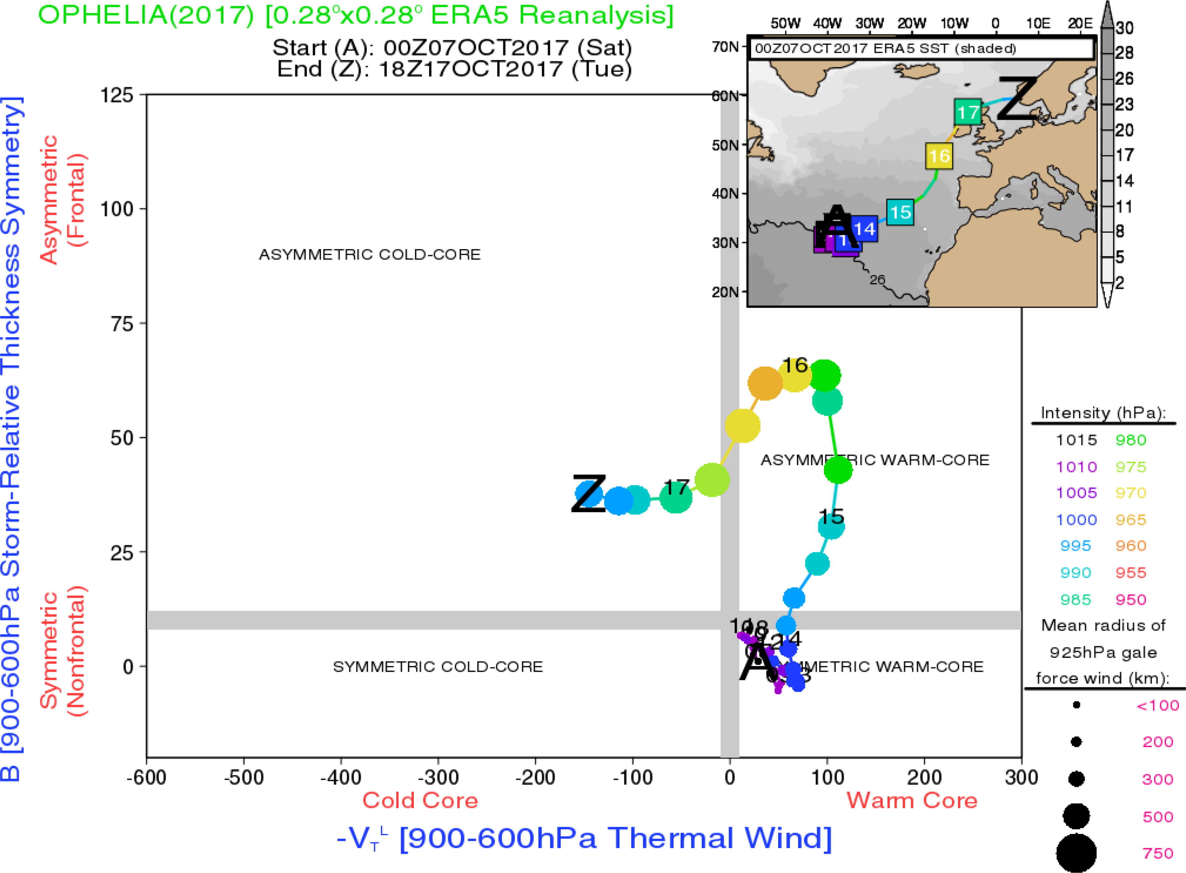
Fig. 2.
Phase space diagram of Ophelia based on ERA5 reanalysis. The dots are plotted every six hours and the numbers labeled in the dots indicate the days of October 2017. The figure is from Hart (2018) and is used with permission.
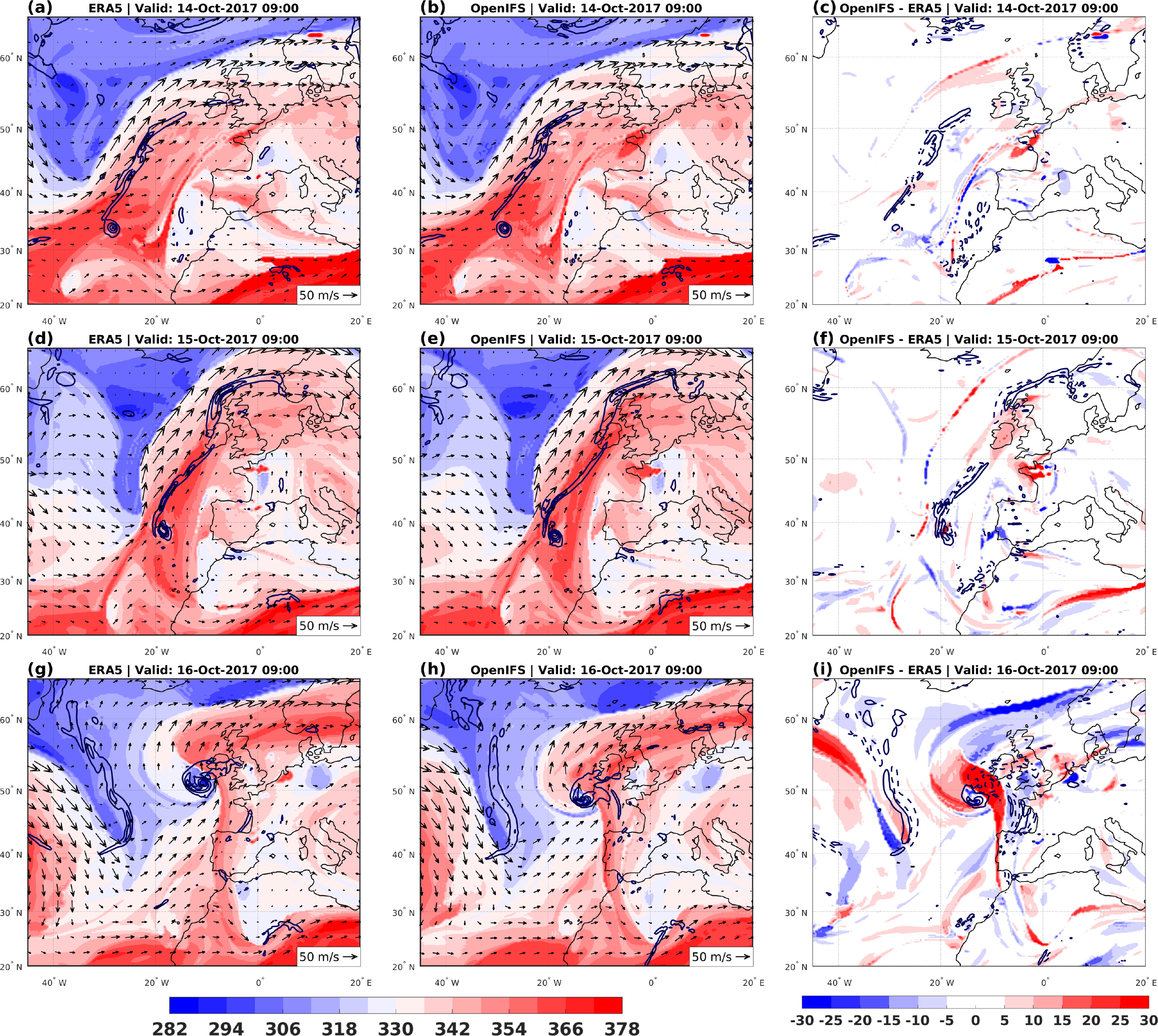
Fig. 3.
Potential temperature (colours, K) and wind (arrows, reference arrow in the lower-right corner) on dynamic tropopause (2.0 PVU), and relative vorticity averaged over 950–850-hPa layer (contours, with 2 × 10⁻⁴ s−1 interval starting from 10−4 s−1) from ERA5 (left column) and OpenIFS (middle column) at 9 UTC 14 October (upper row), 9 UTC 15 October (middle row), and 9 UTC 16 October (bottom row). The difference OpenIFS - ERA5 of potential temperature on 2.0 PVU (colours, with a separate colourbar) and relative vorticity averaged over 950–850-hPa layer (contours) are shown in the right column. In panels (c), (f) and (i), the solid lines show areas where the relative vorticity is higher in OpenIFS than in ERA5, and the dashed lines show the opposite.
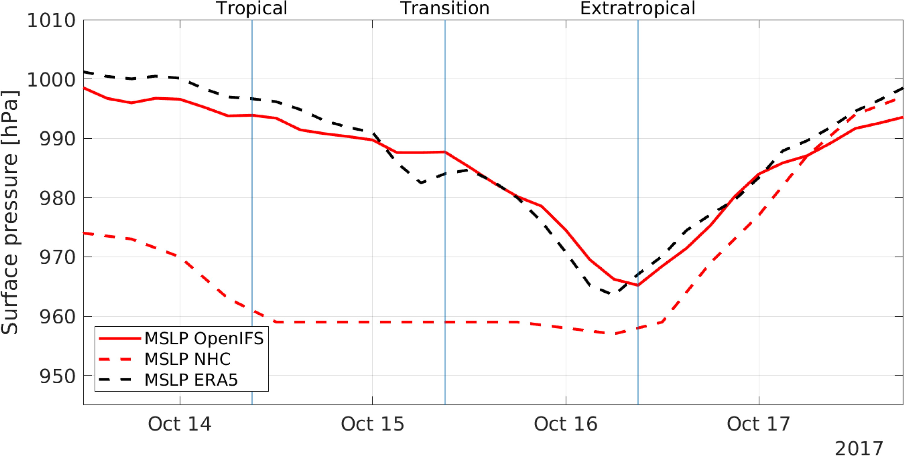
Fig. 4.
Time series of mean sea level pressure at the cyclone centre based on OpenIFS (solid red line), ERA5 reanalysis (dashed black line), and National Hurricane Center best track data (dashed red line). The vertical lines mark the tropical, transition, and extratropical phases of the cyclone.
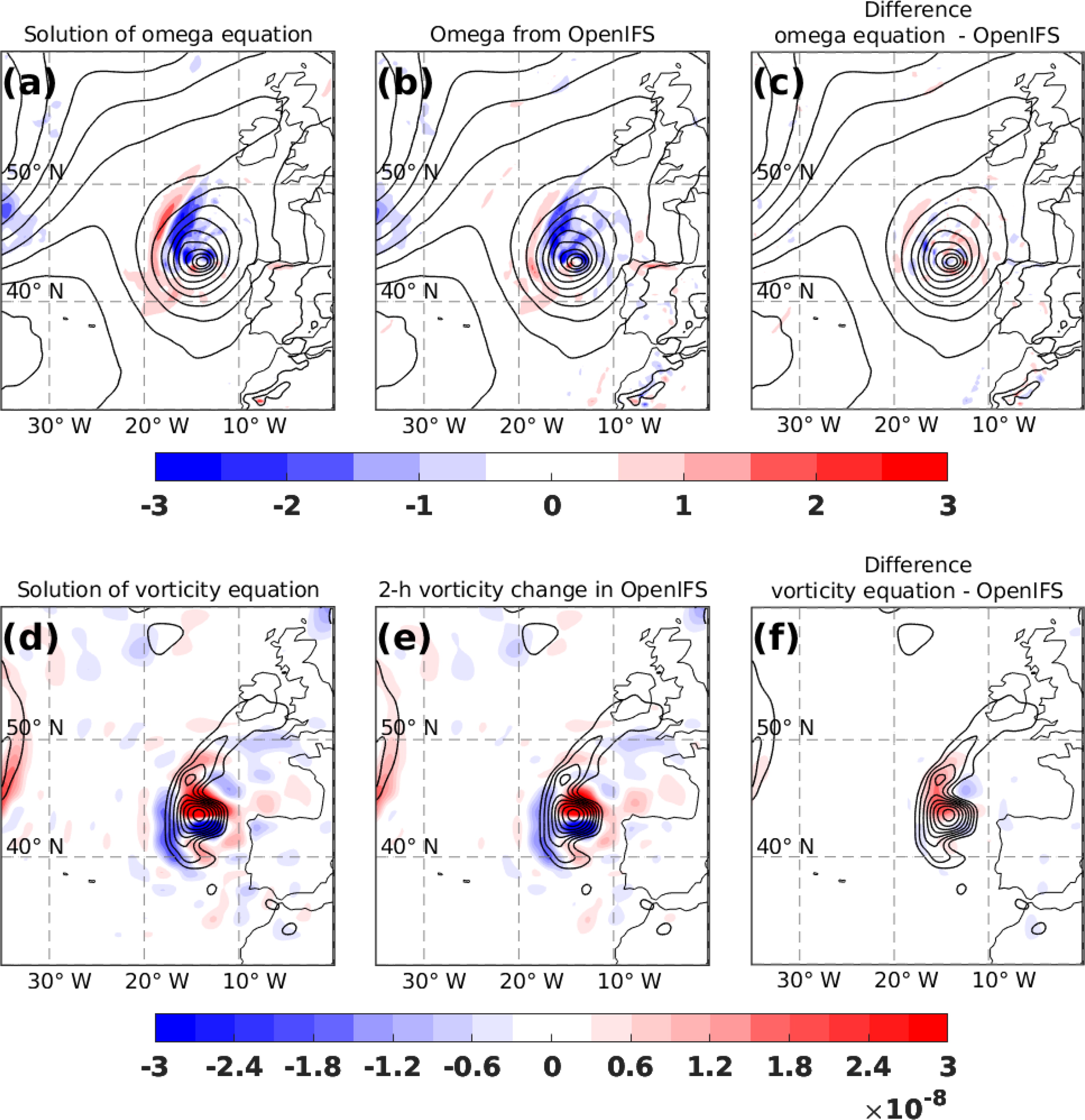
Fig. 5.
The solution of the omega equation (ωTOT) (a), omega directly from OpenIFS output (ωOIFS) (b), and the difference ωTOT - ωOIFS at 700 hPa. The same but for vorticity tendencies at the 900–800-hPa layer is shown in panels (d)–(f). Time is at 21 UTC 15 October 2017. Unit in (a)–(c) is Pa s−1, and in (d)–(f) s−2. Contours in (a)–(c) show mean sea level pressure with 4-hPa interval, and in (d)–(f) relative vorticity averaged over 900–800 hPa starting from 5 × 10⁻⁵ s−1, with 5 × 10⁻⁵ s−1 interval.
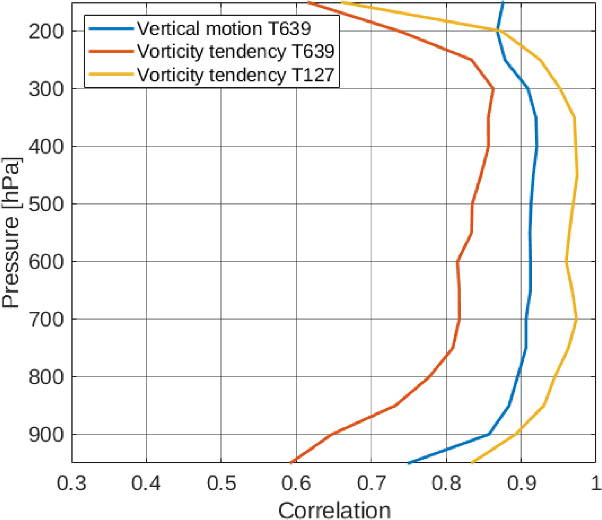
Fig. 6.
Correlation between ωOIFS and the solution of the omega equation (blue), and correlation between and the solution of the vorticity equation (red) as a function of pressure. The values have been calculated from a 10° × 10° moving box centred to the centre of Ophelia, and averaged over the time period 15 UTC 13 October–12 UTC 18 October.
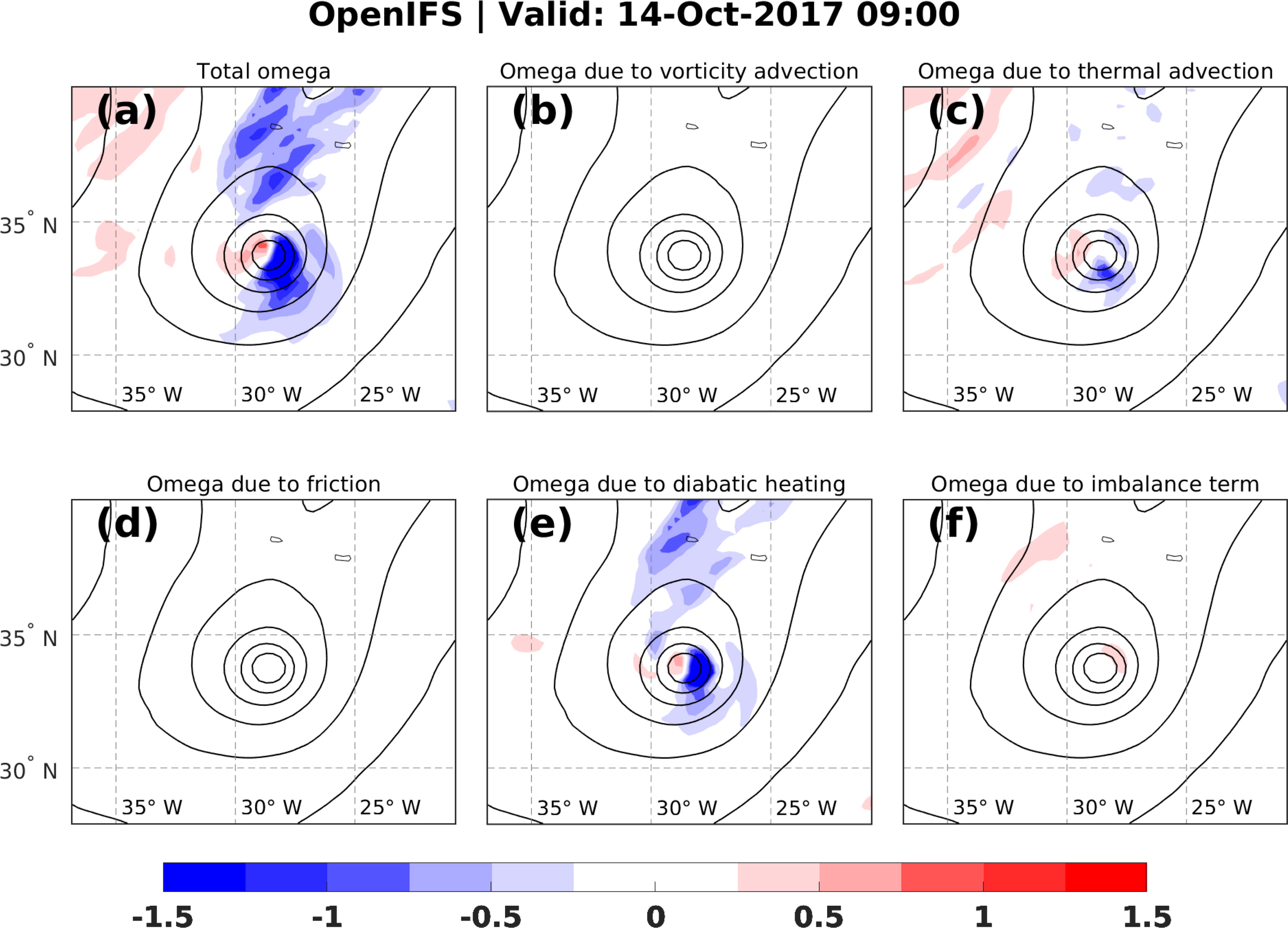
Fig. 7.
Vertical motion (shading, Pa s−1) at 700 hPa at 9 UTC 14 October (tropical phase). The panel (a) shows the total vertical motion due to all five forcing terms [the sum of terms (b)–(f)]. Panels (b)–(f) show the contributions from individual forcing terms: vertical motion due to (b) vorticity advection, (c) thermal advection, (d) friction, (e) diabatic heating, and (f) the imbalance term. The contours show sea level pressure with 4-hPa interval.
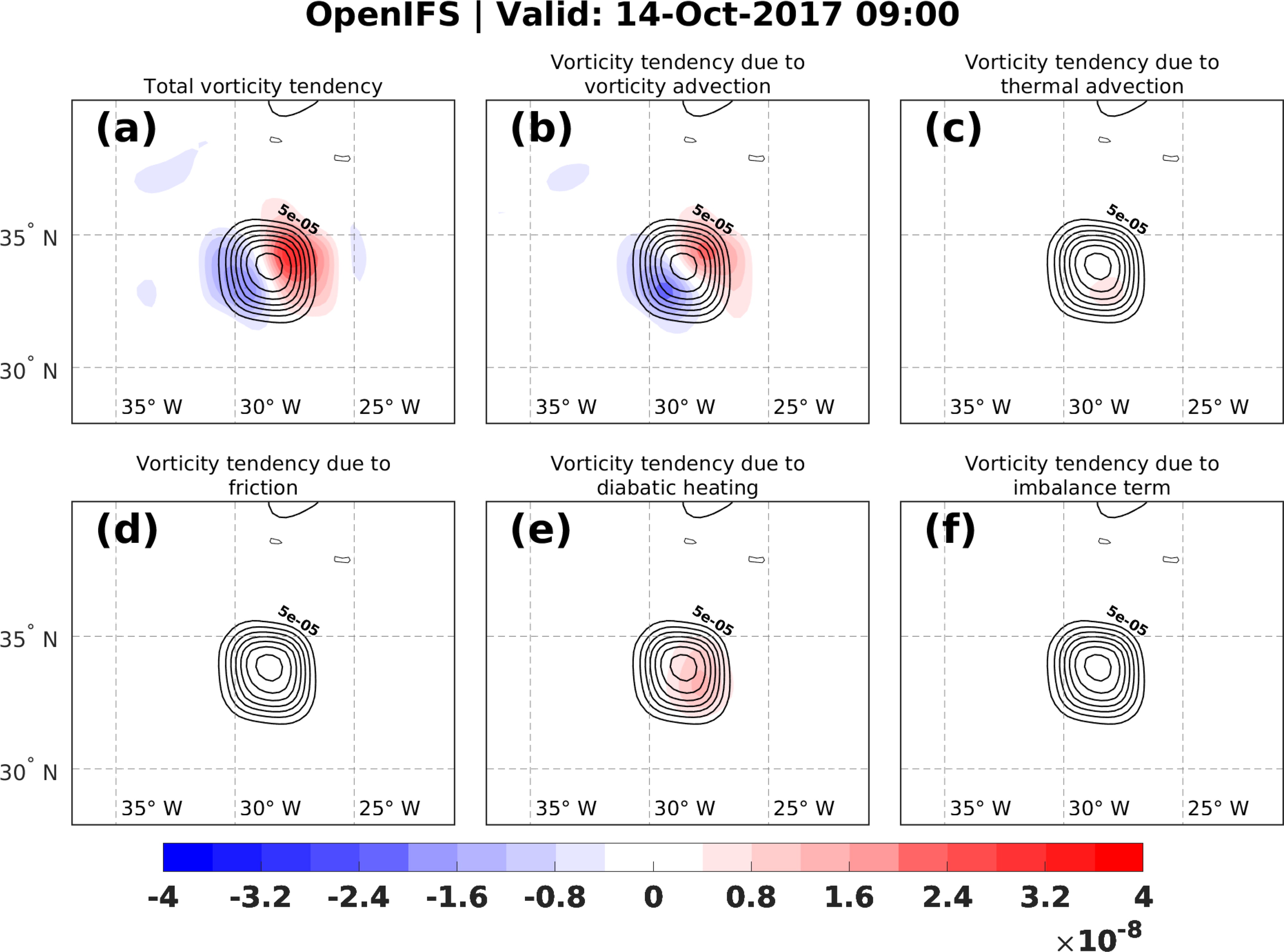
Fig. 8.
Vorticity tendency (shading, s−2) averaged over the 900–800-hPa layer at 9 UTC 14 October (tropical phase). The panel (a) shows the total vorticity tendency due to all five forcing terms [the sum of terms (b)–(f)]. Panels (b)–(f) show the contributions from individual forcing terms: vorticity tendency due to (b) vorticity advection, (c) thermal advection, (d) friction, (e) diabatic heating, and (f) the imbalance term. The contours show relative vorticity, starting from 5 × 10⁻⁵ s−1, with 5 × 10⁻⁵ s−1 interval.
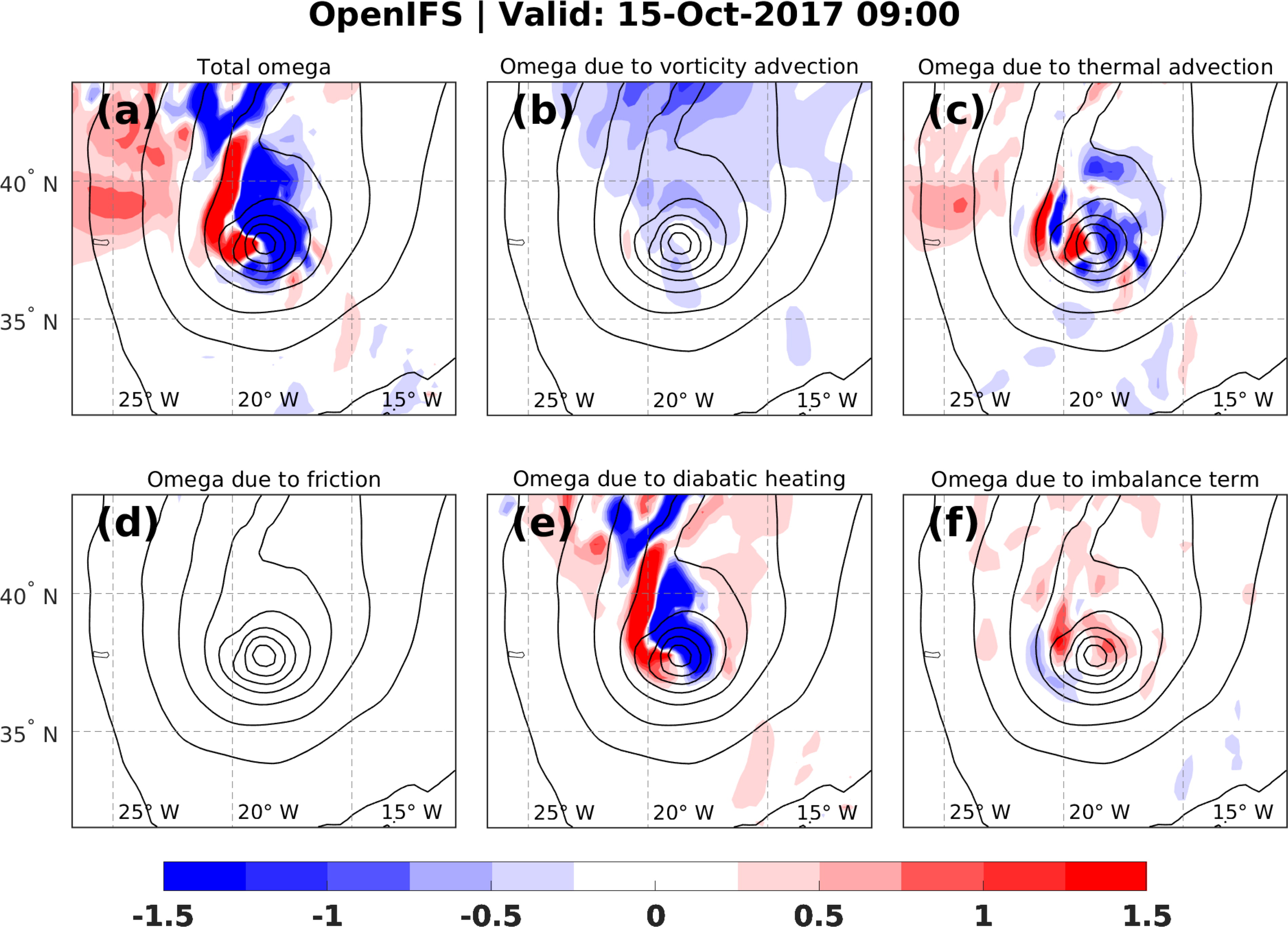
Fig. 9.
As Fig. 7, but at 9 UTC 15 October (transition phase).
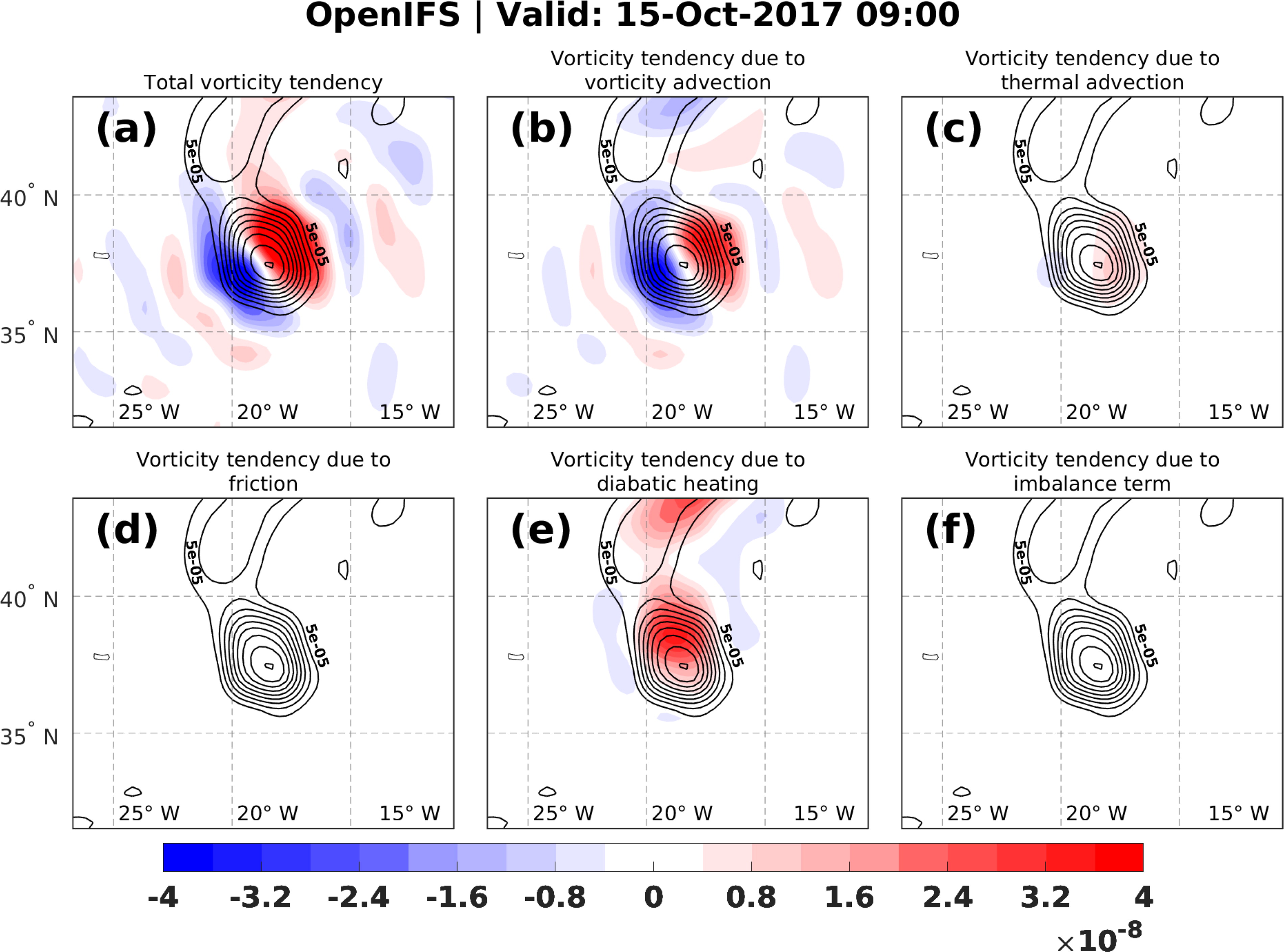
Fig. 10.
As Fig. 8, but at 9 UTC 15 October (transition phase).

Fig. 11.
Potential temperature at 850 hPa (colours, 294 K isentrope contoured with dashed line) at 9 UTC 16 October (extratropical phase) in the OpenIFS simulation (a), and a visible satellite image captured at 1243 UTC 16 October 2017 (b). Contours in (a) represent mean sea level pressure with 4-hPa intervals, and the blue rectangle in (a) marks the area shown in Figs. 12 and 13. Satellite image copyright NERC Satellite Receiving Station, Dundee University, Scotland (http://www.sat.dundee.ac.uk).
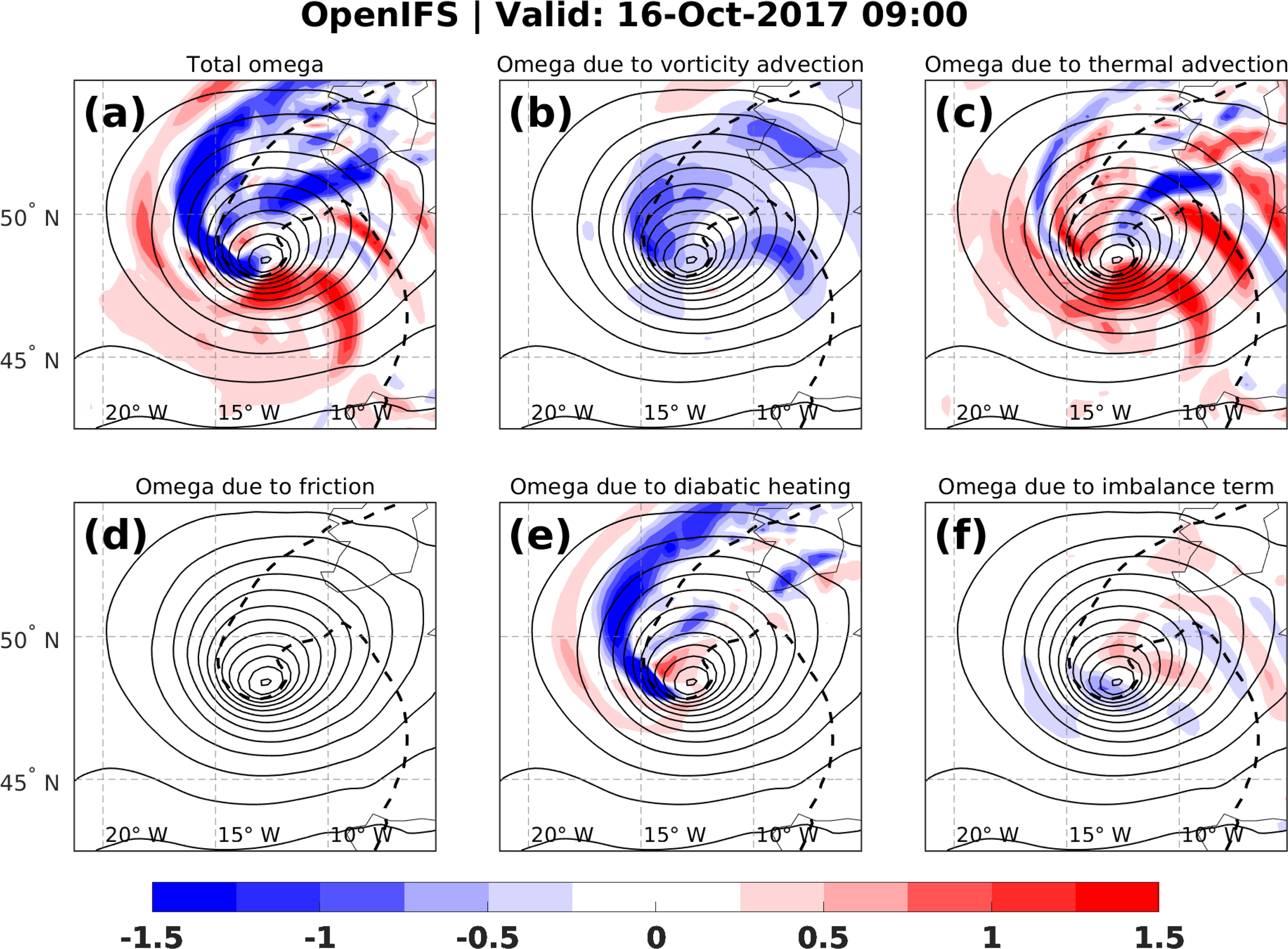
Fig. 12.
As Fig. 7, but at 9 UTC 16 October (extratropical phase). The dashed line shows the 294 K isentrope at 850 hPa.
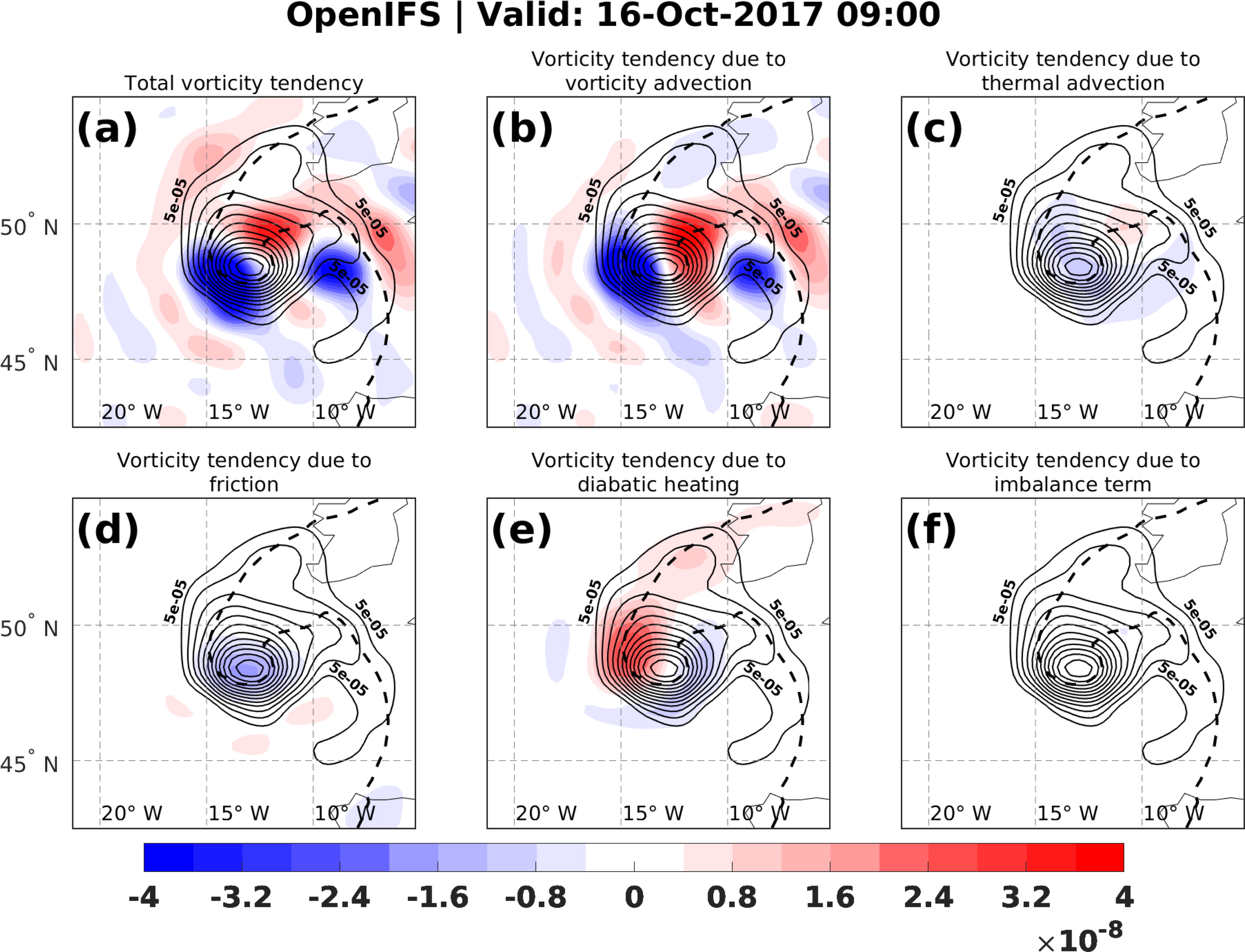
Fig. 13.
As Fig. 8, but at 9 UTC 16 October (extratropical phase). The dashed line shows the 294 K isentrope at 850 hPa.
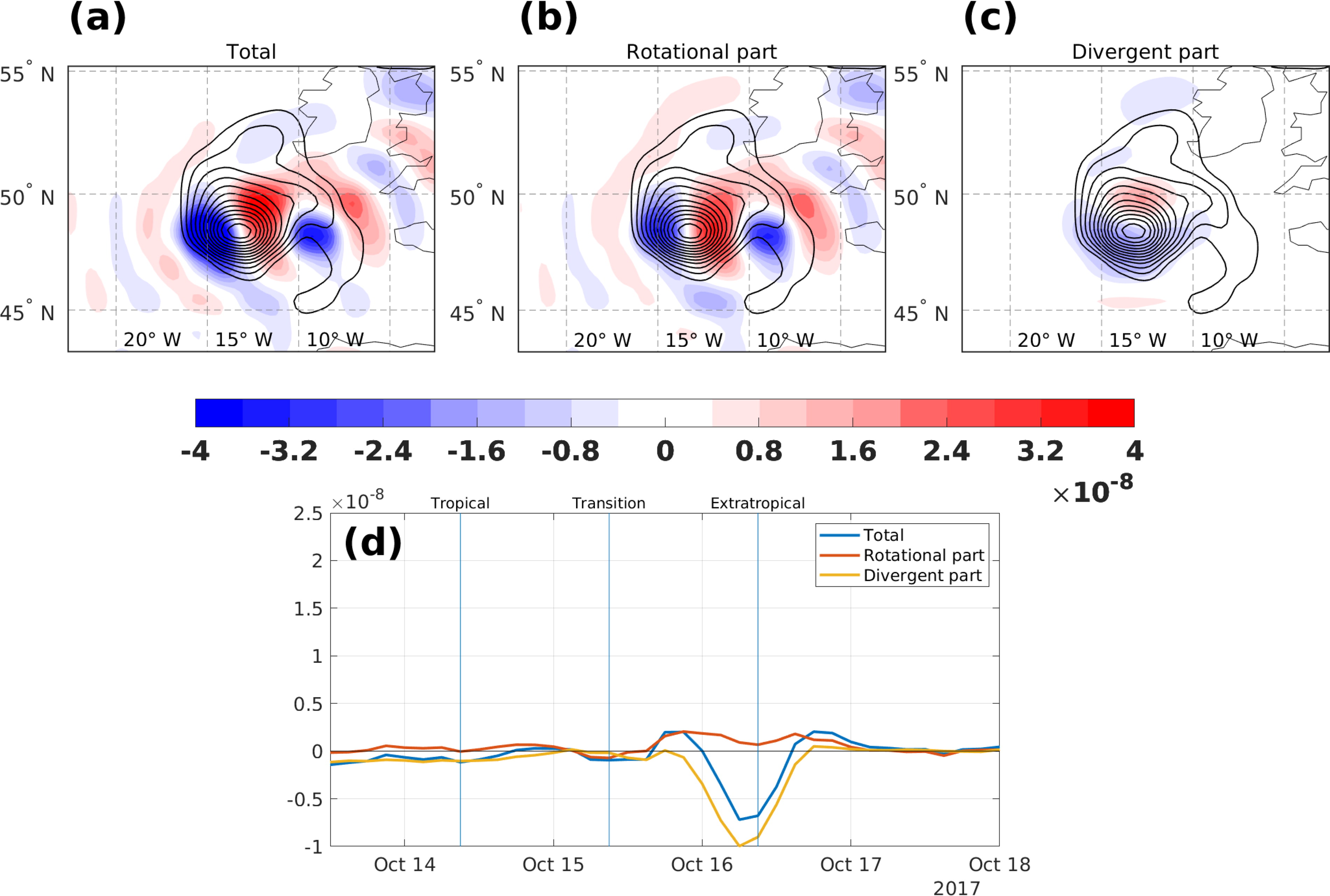
Fig. 14.
Vorticity tendency induced by (a) total vorticity advection, (b) vorticity advection by rotational winds, and (c) vorticity advection by divergent winds at 9 UTC 16 October (extratropical phase). In d), time series of vorticity advection by rotational winds (red), divergent winds (yellow), and total winds (blue) averaged over 1.5° circle are shown. The times of tropical, transition, and extratropical phases have been marked with vertical lines in (d).
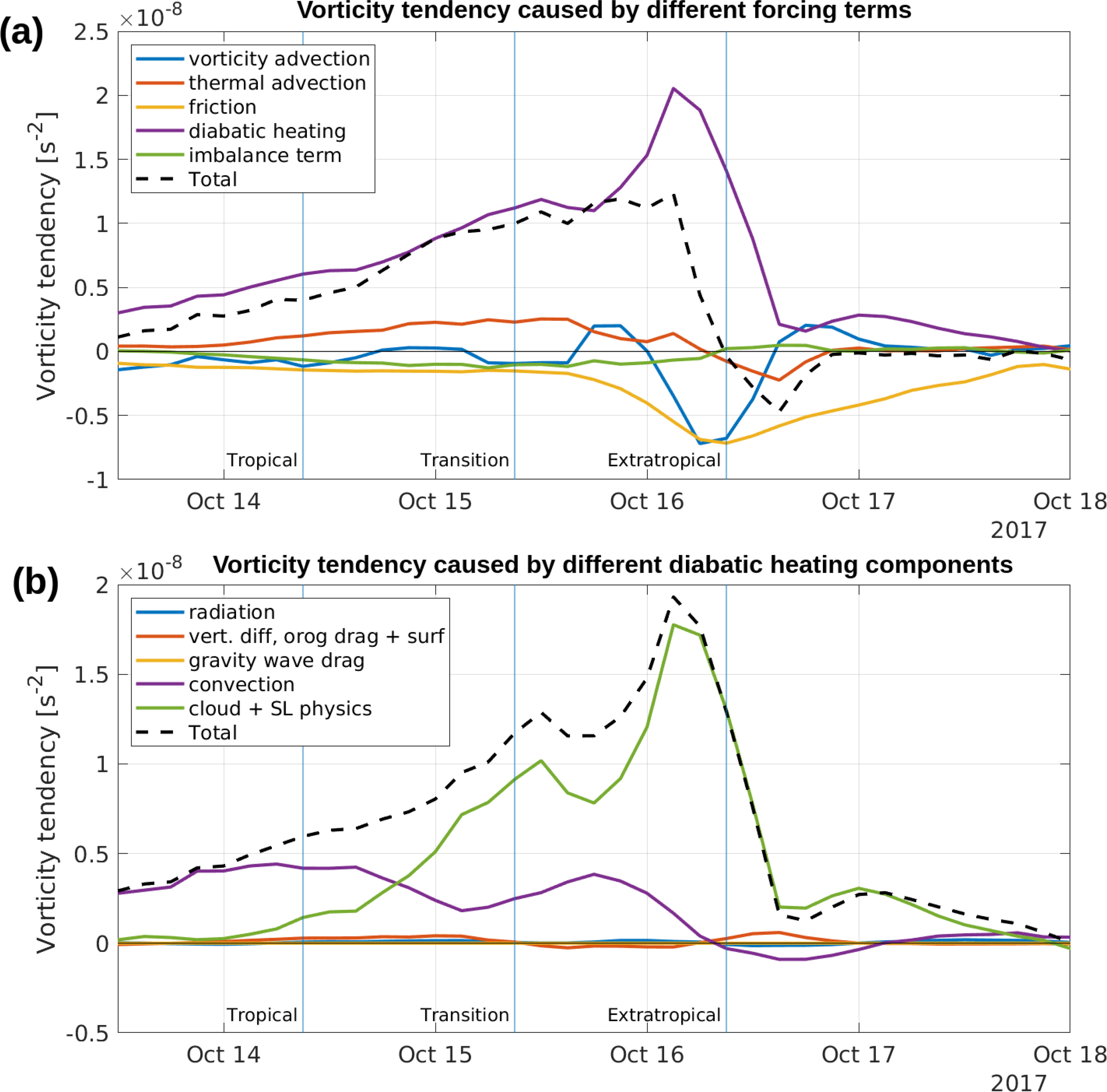
Fig. 15.
Time series of vorticity tendencies caused by (a) different forcing terms and (b) different diabatic heating components. The values have been averaged over the 900–800-hPa layer and over a circular area with a 1.5° radius centred on the maximum of the T127 vorticity field. All values are 12-hour moving averages. The times of tropical, transition, and extratropical phases have been marked with vertical lines.
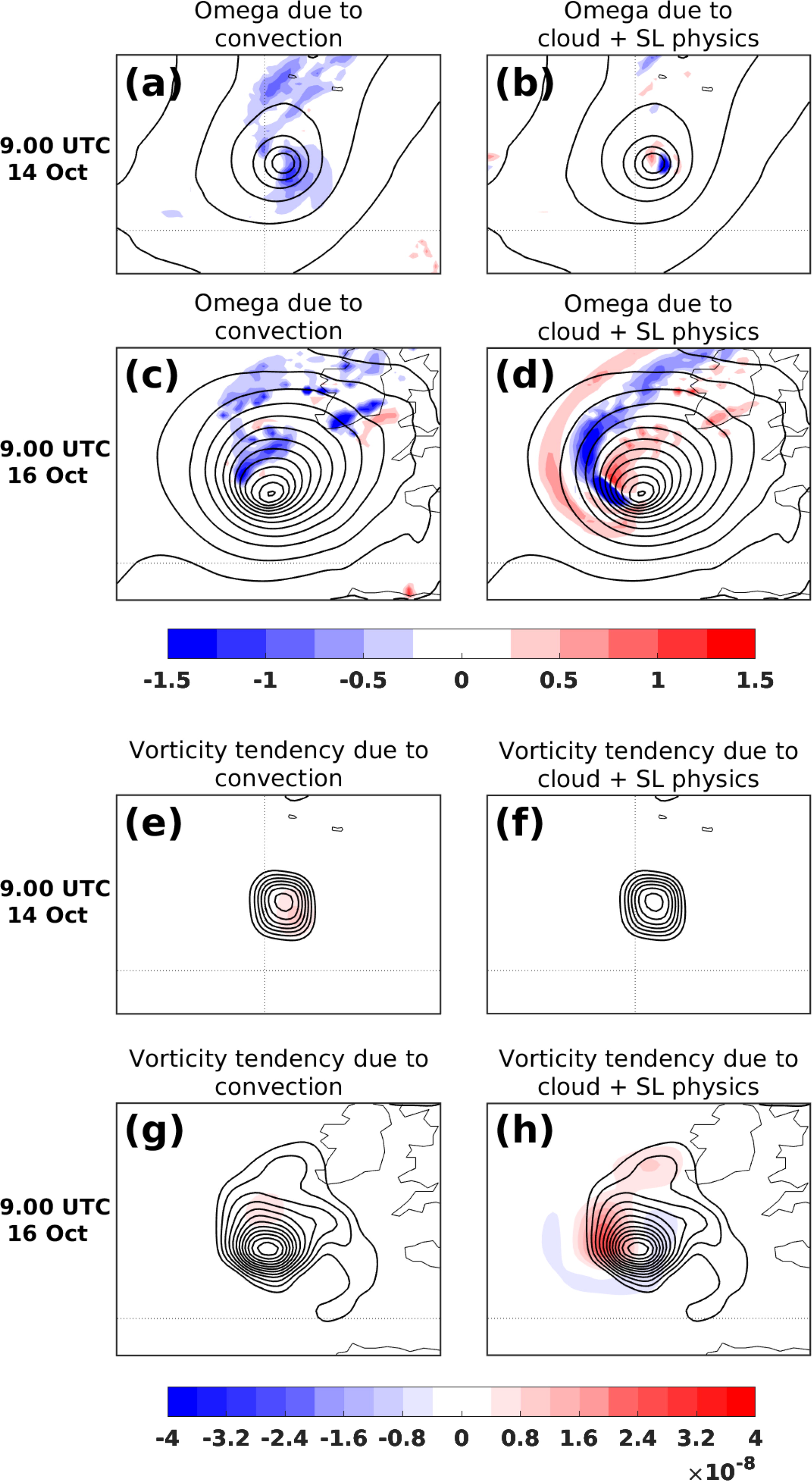
Fig. 16.
Panels (a) – (d) show vertical motion (shading, Pa s−1) at 700 hPa and sea level pressure (contours, with 4-hPa interval), and panels (e) – (h) show vorticity tendency (shading, s−2) and relative vorticity (contours, starting from 5 × 10⁻⁵ s−1, with 5 × 10⁻⁵ s−1 interval) averaged over the 900–800-hPa layer. The left-hand panels [(a), (c), (e), and (g)] show vertical motion and vorticity tendency due to the convection parametrization, and the right-hand panels [(b), (d), (f) and (h)] show vertical motion and vorticity tendency due to the microphysics parametrization. The upper panels in both vertical motion [(a) and (b)] and in vorticity tendency [(e) and (f)] show the situation at 9 UTC 14 October (tropical phase), and the lower panels [(c), (d), (g) and (h)] at 9 UTC 16 October (extratropical phase). The size of the panels is 16° longitude by 12° latitude, centred on the cyclone vorticity maximum.