Have a personal or library account? Click to login
Analyses of the relationship between drought occurrences and their causal factors in Tigray Region, Northern Ethiopia Cover

Analyses of the relationship between drought occurrences and their causal factors in Tigray Region, Northern Ethiopia

By: ,   and    
Open Access
|Jan 2020

Figures & Tables

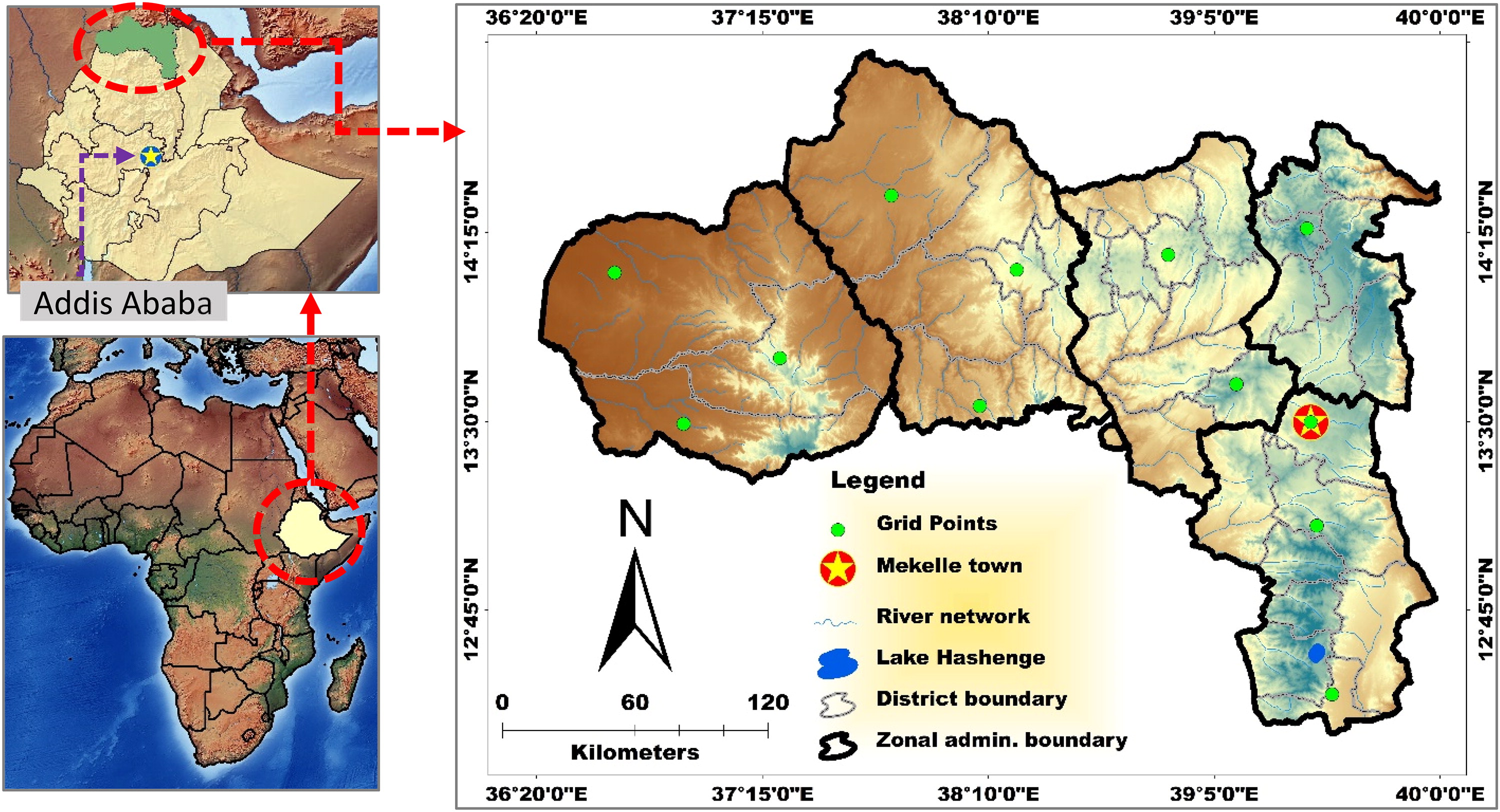
Fig. 1.

Map of the study area.
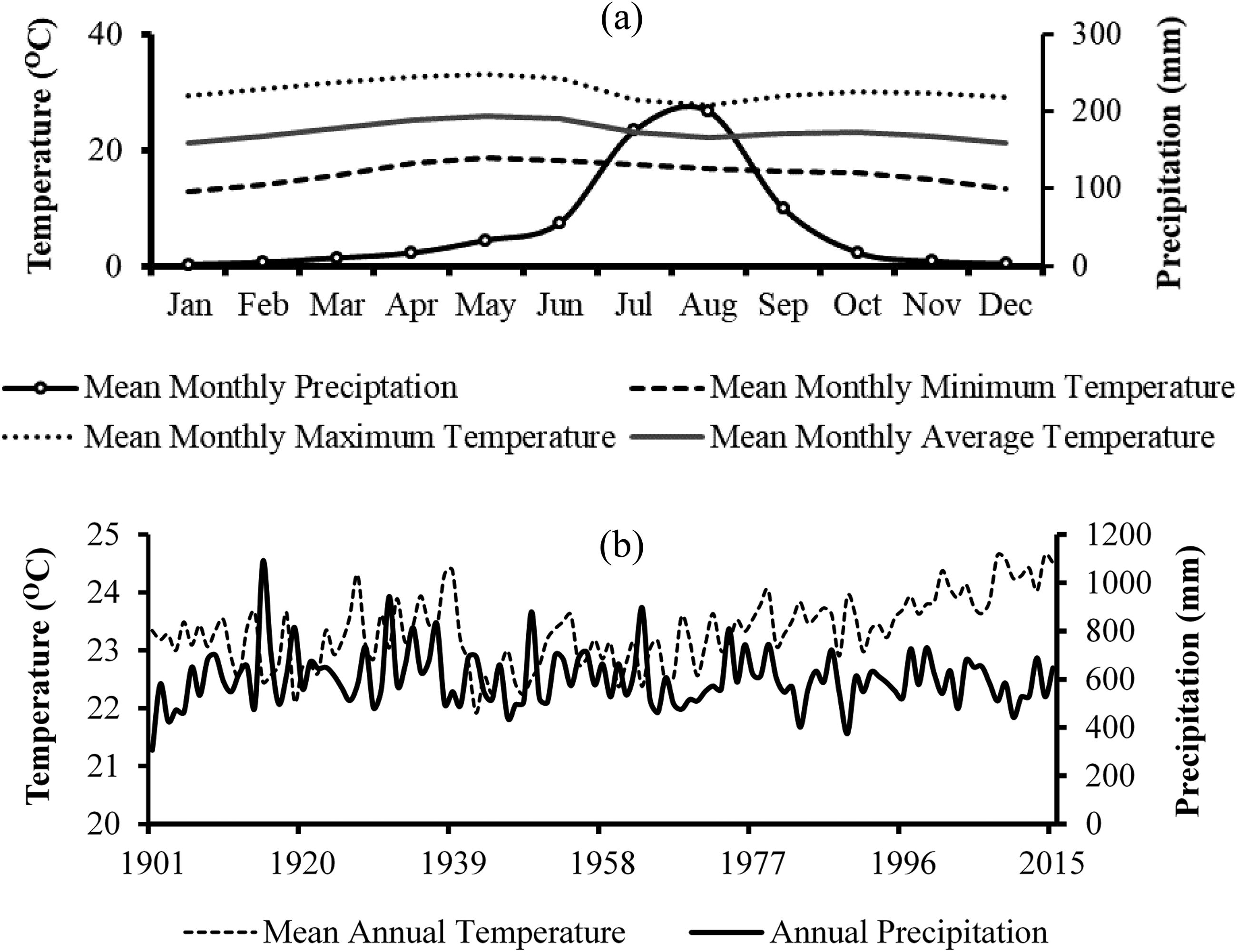
Fig. 2.

Mean monthly (a) and mean annual (b) precipitation and temperature of the study area for the period 1901 to 2016.
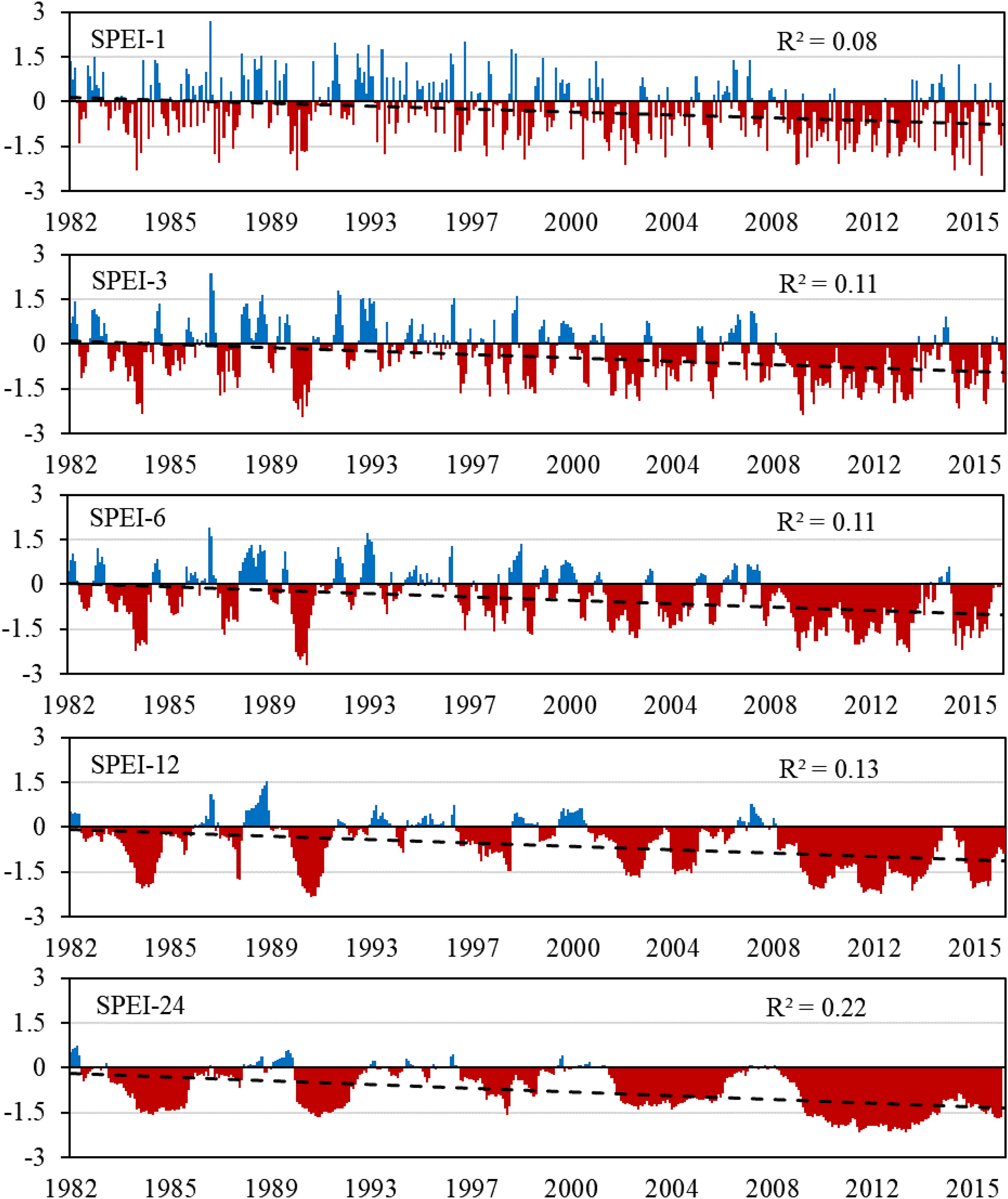
Fig. 3.

Temporal pattern of SPEI at 1-month, 3-month, 6-month, 12-month and 24-month time scales (1982 to 2016).

Table 1.

Test of randomness and the product-moment correlation coefficient values representing the trend of drought conditions in Tigray region at 1-month, 3-month, 6-month, 12-month and 24-month time scale (1982–2016).
Time scaleRun’s test (z)Correlation coefficient (r)p-value1-month−4.01−0.274**0.0003-month−12.21−0.330**0.0006-month−15.24−0.335**0.00012-month−17.29−0.367**0.00024-month−19.25−0.472**0.000

** Correlation is significant at the 0.01 level (2-tailed).

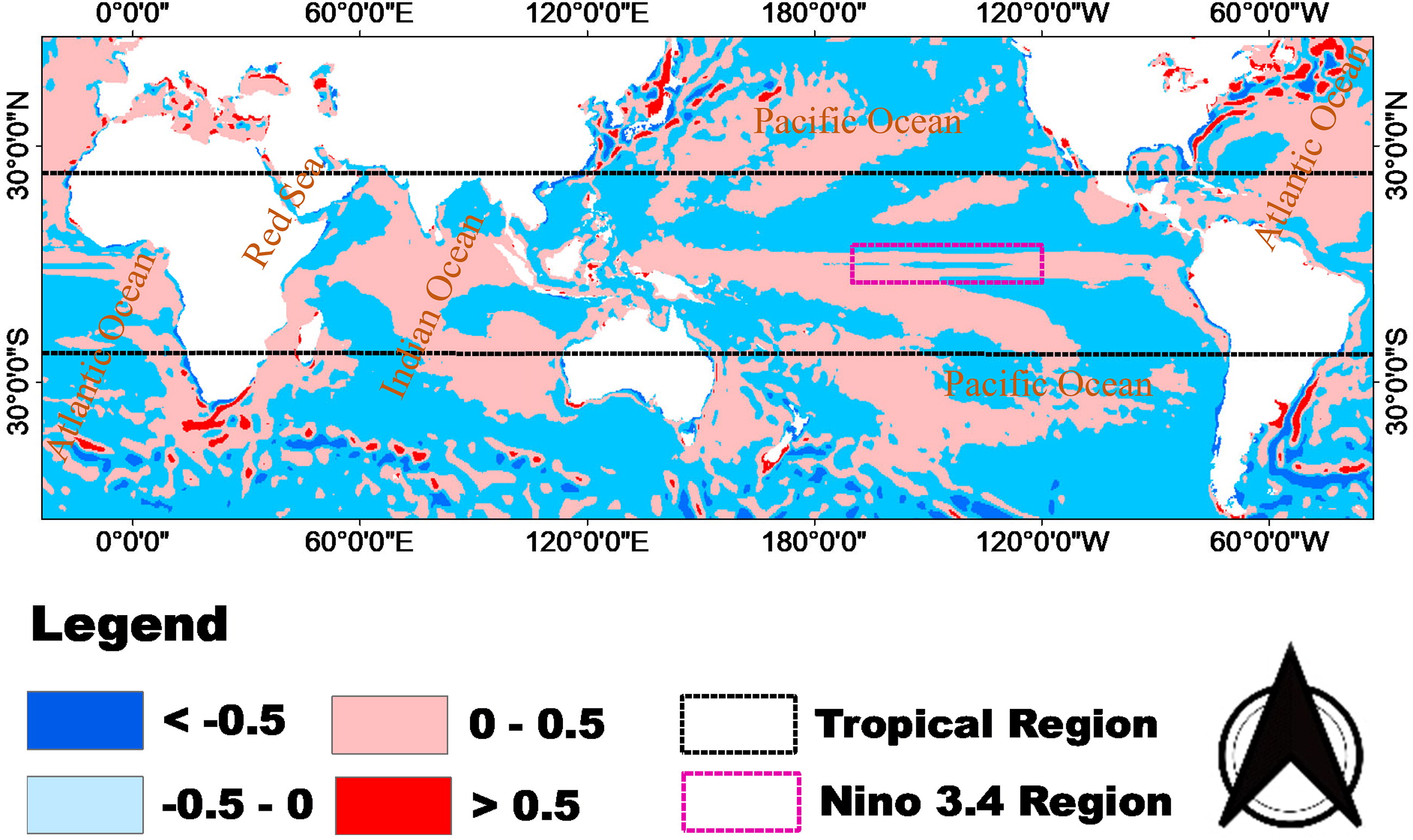
Fig. 4.

Map of sampled tropical Indian Ocean, tropical Atlantic Ocean, tropical Pacific Ocean, the Red Sea and Nino 3.4 regions (12-month average global SSTAs for the period 1982 to 2016).

Table 2.

Trend test summary of the global and local factors used in drought causation analyses (z = run’s test, r = Pearson’s correlation coefficient, p = probability-value) for the period 1982 to 2016.
Climate control factors1-month3-month6-month12-month24-monthzrpzrpzrpzrpzrpTropical Indian Ocean (SSTA)−13.480.63**0.000−16.550.69**0.000−18.530.74**0.000−18.860.79**0.000−19.250.86**0.000Tropical Atlantic Ocean (SSTA)−13.970.613**0.000−16.450.651**0.000−17.740.692**0.000−18.66.747**0.000−18.950.802**0.000Tropical Pacific Ocean (SSTA)−14.270.49**0.000−15.570.53**0.000−17.640.58**0.000−18.660.61**0.000−18.540.67**0.000Nino 3.4 (SSTA)−17.88−0.070.17−18.41−0.070.18−18.23−0.06**0.19−18.76−0.060.22−18.640.0530.000Red Sea (SSTA)−9.380.54**0.000−14.500.63**0.000−16.070.69**0.000−18.270.76**0.000−18.240.80**0.000SOI−7.910.18**0.000−14.400.21**0.000−15.970.23**0.000−17.670.26**0.000−18.440.33**0.000NDVI−11.220.59**0.000−15.740.66**0.000−19.510.76**0.000−19.850.88**0.000−19.750.89**0.000Albedo−19.25−0.75**0.000−19.20−0.78**0.000−19.71−0.81**0.000−19.75−0.85**0.000−19.75−0.87**0.000

** Correlation is significant at the 0.01 level (2-tailed).

Fig. 5.

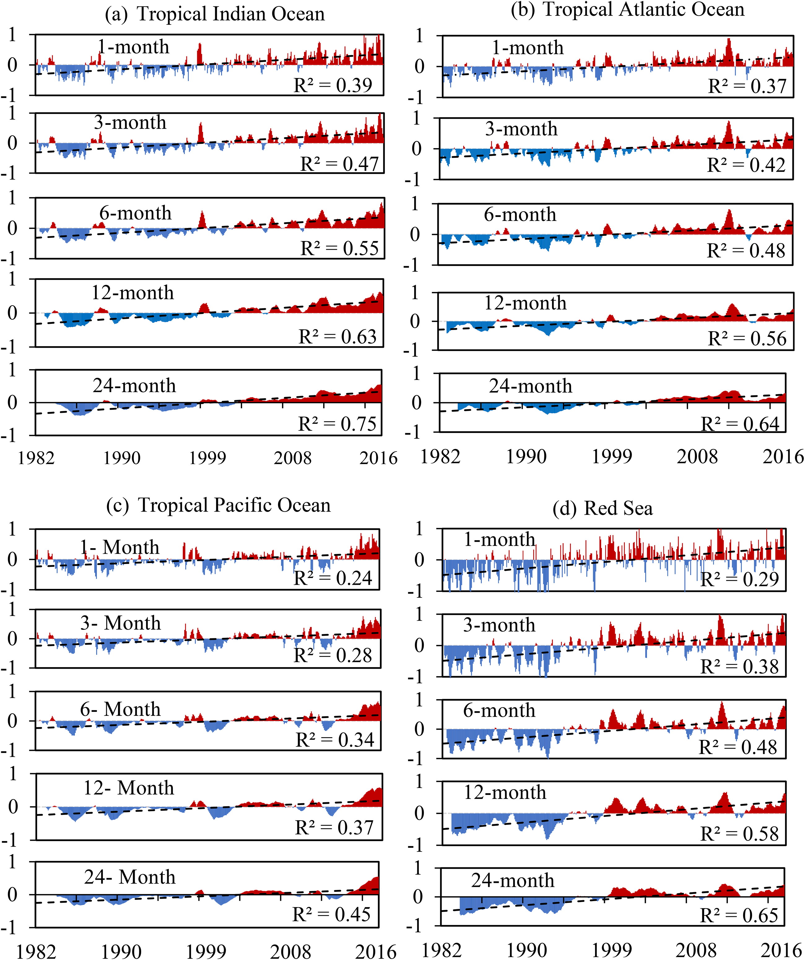
Running means of the sea surface temperature anomalies for the (a) tropical Indian Ocean, (b) tropical Atlantic Ocean, (c) tropical Pacific Ocean and (d) Red Sea region on 1-month, 3-month, 6-month, 12-month and 24-month basis.
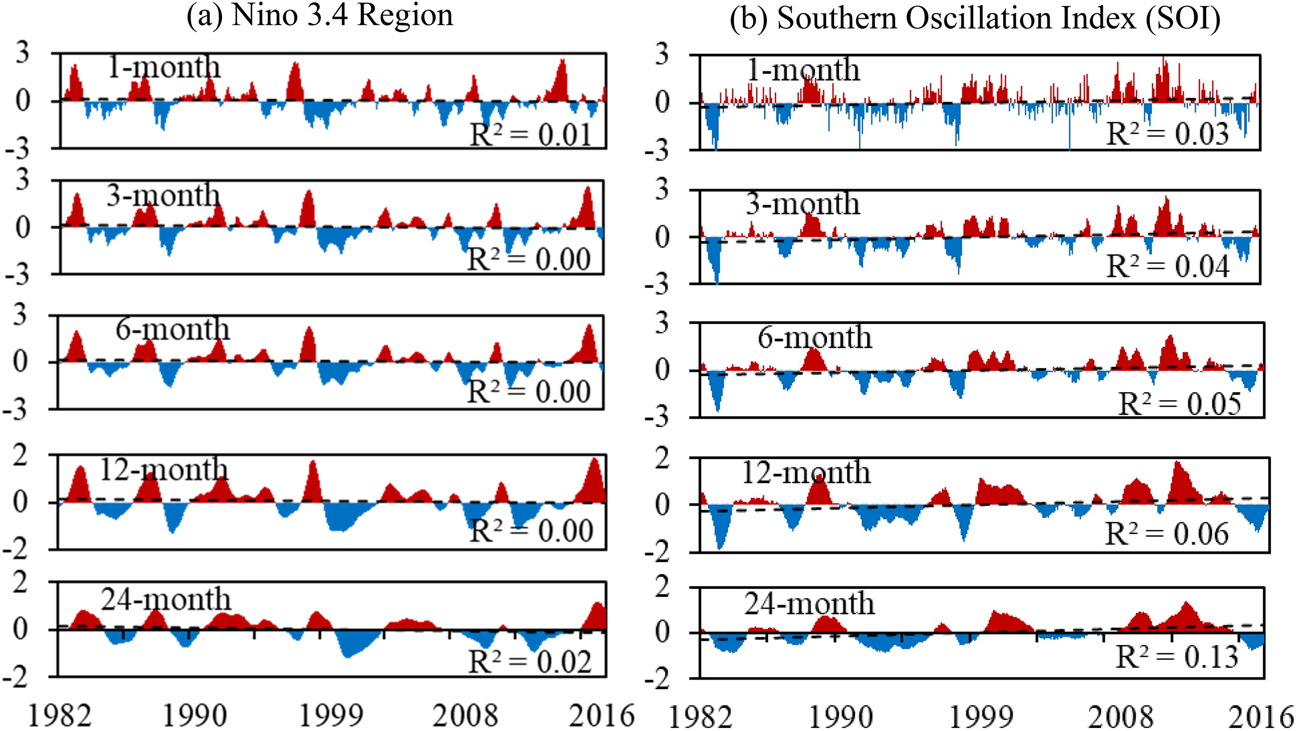
Fig. 6.

Running means of the (a) Nino 3.4 region surface temperature anomaly and (b) Southern Oscillation Index (SOI) on 1-month, 3-month, 6-month, 12-month and 24-month basis.
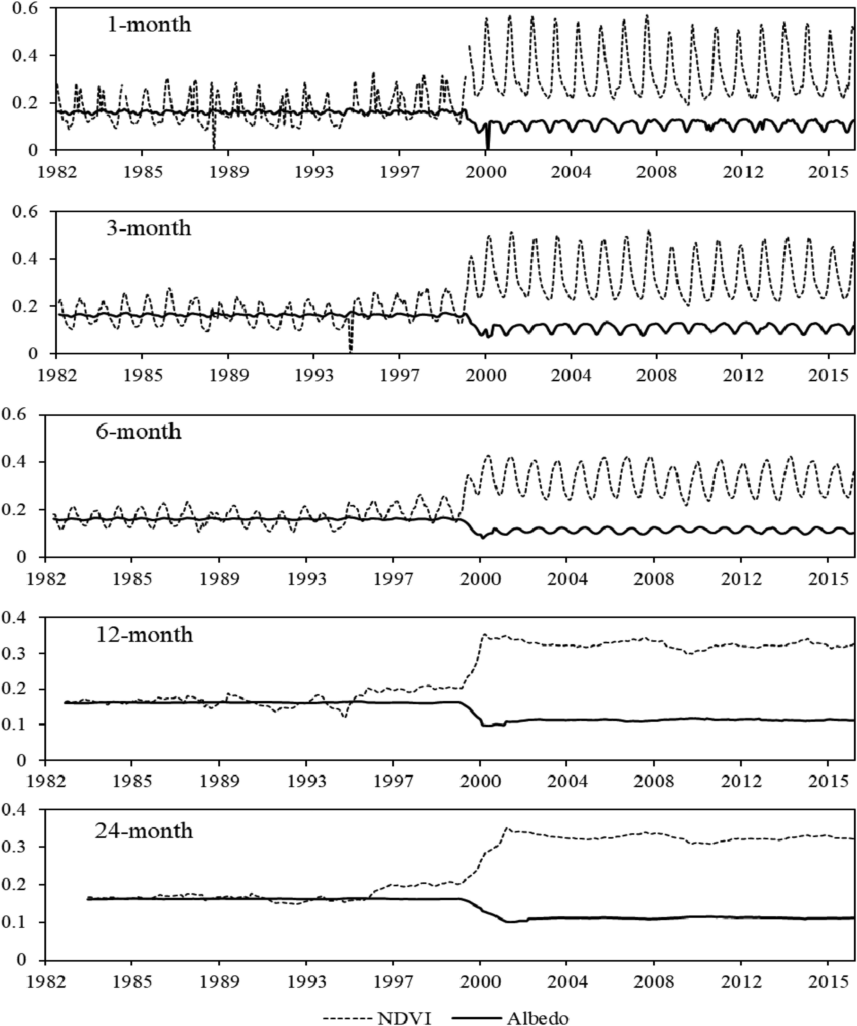
Fig. 7.

Temporal pattern of average NDVI and Albedo at 1-month, 3-month, 6-month, 12-month and 24-month time scales.

Table 3.

Correlation coefficient (r) values between zero-lag SPEI and the local and global climate controlling factors at 1-month, 3-month, 6-month, 12-month and 24-month time scales for the period 1982 to 2016.
Climate control factors1-monthp-value3-monthp-value6-monthp-value12-monthp-value24-monthp-valueTropical Indian Ocean (SSTA)−0.242**0.000−0.280**0.000−0.282**0.000−0.340**0.000−0.490**0.000Tropical Atlantic Ocean (SSTA)−0.208**0.000−0.269**0.000−0.247**0.000−0.302**0.000−0.413**0.000Tropical Pacific Ocean (SSTA)−0.153**0.002−0.178**0.000−0.200**0.000−0.268**0.000−0.328**0.000Red Sea (SSTA)−0.140**0.004−0.172**0.000−0.135**0.006−0.133**0.007−0.207**0.000Nino 3.4 (SSTA)0.0210.672−0.0160.739−0.100*0.043−0.148**0.003−0.0760.129SOI−0.115*0.018−0.143**0.003−0.098*0.046−0.0410.413−0.165**0.001NDVI−0.196**0.000−0.244**0.000−0.263**0.000−0.283**0.000−0.374**0.000Albedo0.117*0.0170.179**0.0000.208**0.0000.287**0.0000.390**0.000

* Correlation is significant at the 0.05 level (2-tailed).

** Correlation is significant at the 0.01 level (2-tailed).

Fig. 8.

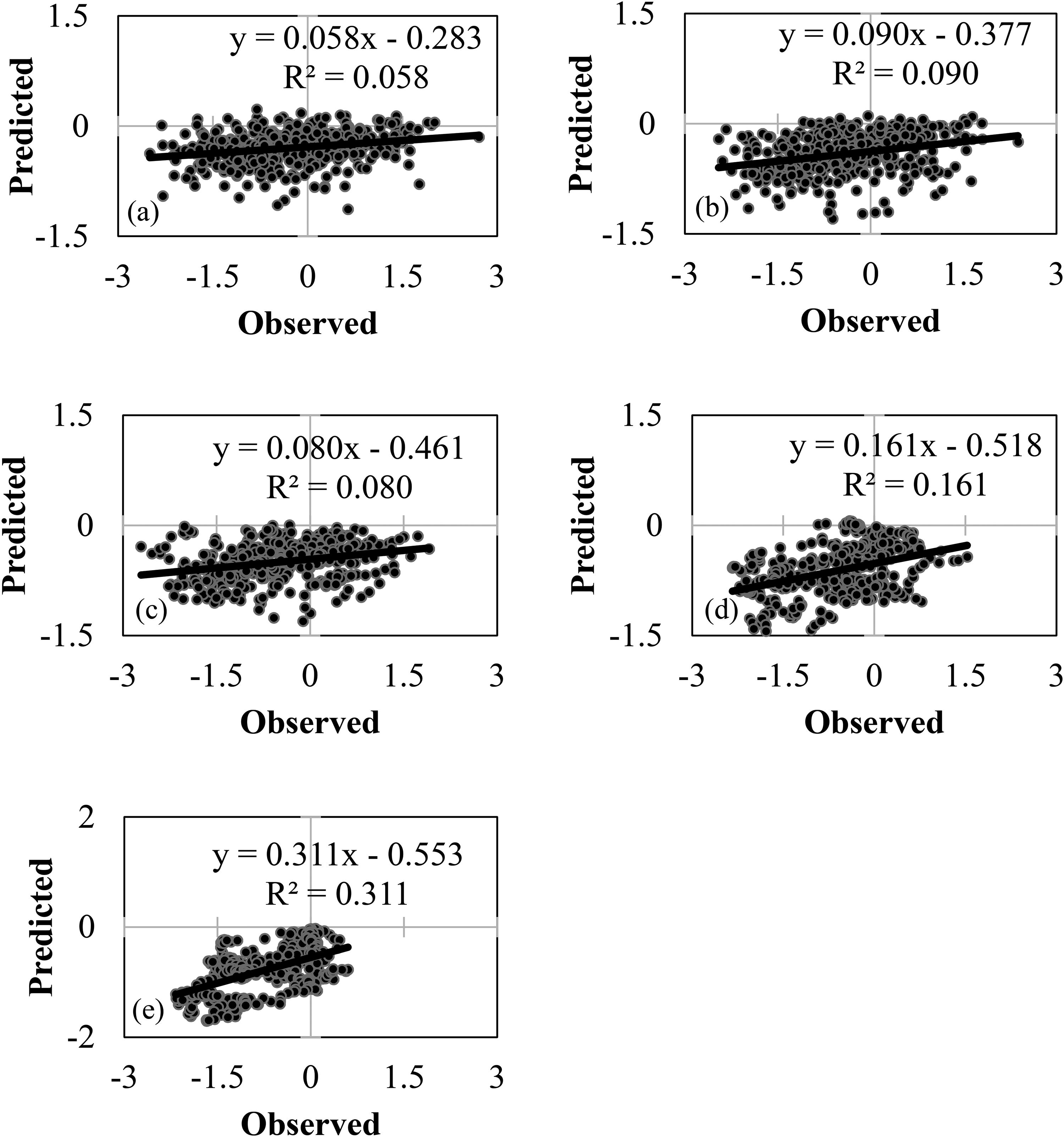
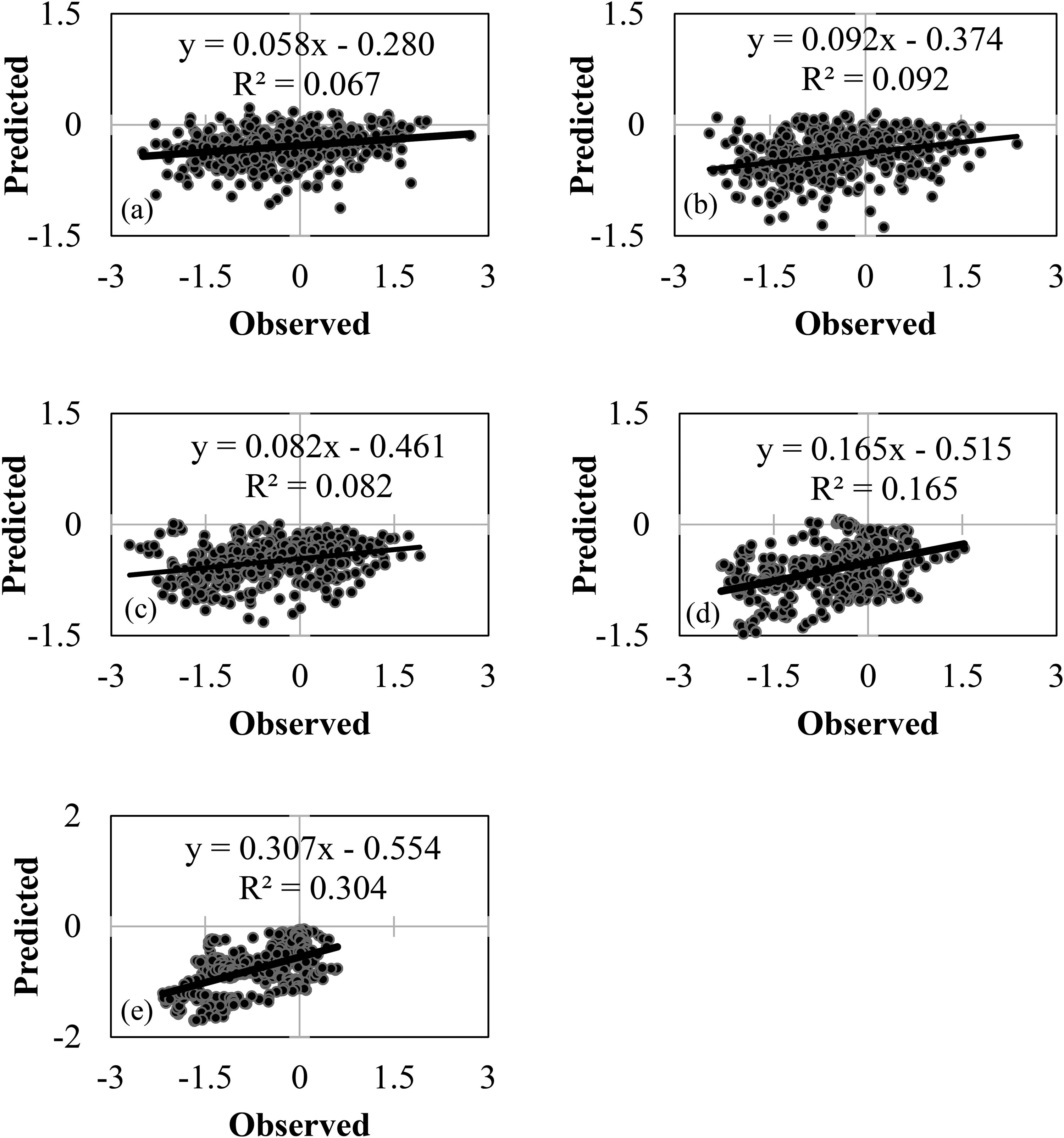
Scatter plots showing the zero-time-lag observed SPEI against predicted SPEI values at (a)1-month, (b) 3-month, (c) 6-month, (d) 12-month and (e) 24-month time scales.

Table 4.

Correlation coefficient (r) values between time-lagged SPEI and the local and global climate controlling factors at 1-month, 3-month, 6-month, 12-month and 24-month time scales for the period 1982 to 2016.
Climate control factors1-monthp-value3-monthp-value6-monthp-value12-monthp-value24-monthp-valueTropical Indian Ocean (SSTA)−0.240**0.000−0.303**0.000−0.286**0.000−0.344**0.000−0.486**0.000Tropical Atlantic Ocean (SSTA)−0.221**0.000−0.253**0.000−0.248**0.000−0.300**0.000−0.403**0.000Tropical Pacific Ocean (SSTA)−0.171**0.000−0.217**0.000−0.219**0.000−0.278**0.000−0.332**0.000Red Sea (SSTA)−0.137**0.005−0.153**0.002−0.142**0.004−0.136**0.006−0.202**0.000Nino 3.4 (SSTA)0.0300.5380.0010.982−0.097*0.048−0.166**0.001−0.0870.082SOI−0.111*0.024−0.139**0.004−0.0730.136−0.0210.667−0.149**0.003NDVI−0.148**0.003−0.198**0.000−0.216**0.000−0.273**0.000−0.365**0.000Albedo0.143**0.0030.175**0.0000.206**0.0000.281**0.0000.381**0.000

* Correlation is significant at the 0.05 level (2-tailed).

** Correlation is significant at the 0.01 level (2-tailed).

Fig. 9.

Scatter plots showing the time-lagged observed SPEI against predicted SPEI values at (a)1-month, (b) 3-month, (c) 6-month, (d) 12-month, (e) 24-month time scales.

Language: English
Page range: 1718937 - 1718937
Published on: Jan 1, 2020
Published by: Stockholm University Press
In partnership with: Paradigm Publishing Services

© 2020 A.S. Tefera, J.O. Ayoade, N.J. Bello, published by Stockholm University Press
This work is licensed under the Creative Commons Attribution 4.0 License.