Have a personal or library account? Click to login
Nonlinear interaction of gravity and acoustic waves Cover

Nonlinear interaction of gravity and acoustic waves

Open Access
|Jan 2020

Figures & Tables

Table 1.

Definition of variables, symbols and operators.
xEastward distanceyNorthward distancezAltitudetTimeuZonal windvMeridional windwVertical windV=(u,v)THorizontal wind vectorpPressureρDensityTTemperatureRGas constant for dry aircpSpecific heat at constant pressurecvSpecific heat at constant volumeγ=cp/cvκ=R/cpT0=243.878 KTemperature of the isothermal basic stateLx=4×10⁷cos(ϕ0) mZonal periodLy=107 mMeridional periodzT = 18,000 mModel’s topΩ=2π/(24×60×60) s−1Earth’s rotation rateϕ0=π/4Central latitude of f planef=2Ωsin(ϕ0)Coriolis parameterg = 9.8 m s−2Earth’s gravitational accelerationCS=γRT0Linear sound wave speedV·h=uxh+vyh·V=xu+yvHorizontal divergence
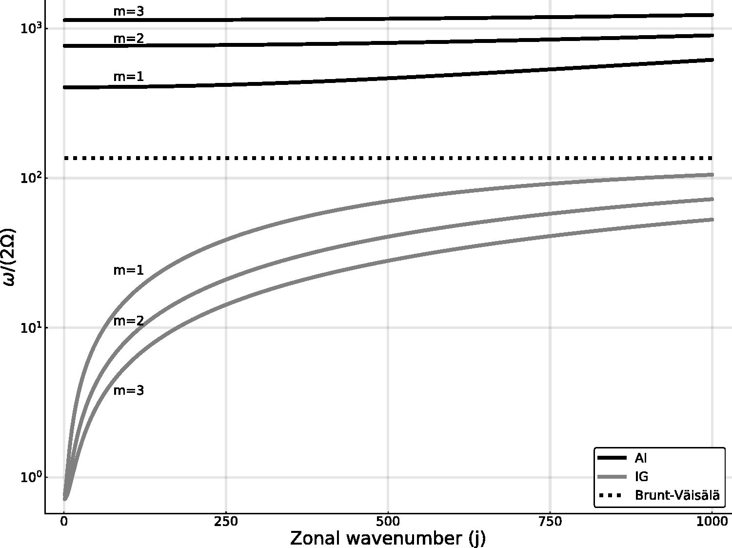
Fig. 1.

Dispersion curves of inertia-acoustic (AI) and inertia-gravity (IG) waves corresponding to the first three baroclinic modes m = 1, 2, 3. All the curves are referred to the meridional index n = 1.
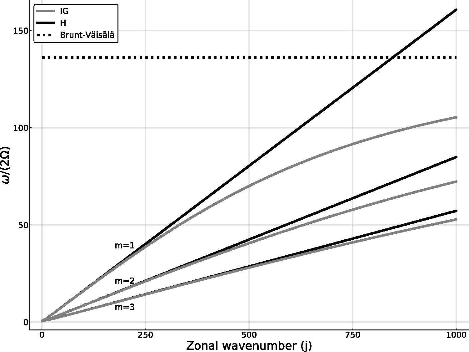
Fig. 2.

Similar to Fig. 1, but only for the inertia-gravity waves (IG) and their corresponding dispersion curves obtained by hydrostatic approximation (H).

Table 2.

Representative examples of interacting triads involving inertia-acoustic (IA) and inertia-gravity modes (IG).

TriadMode aMode bMode cωaωbωcδabciσaiσbiσc1(1, 1, 1, IA)(339, 1, 2, IG)(340, 1, 1, IA)5.89E–024.10E–036.30E–023.31E–05–3.11E–01–2.16E–02–3.33E–012(170, 1, 2, IG)(169, 1, 2, IG)(339, 1, 2, IG)2.09E–032.08E–034.10E–03–6.94E–05–3.37E + 02–3.35E + 02–6.73E + 023(169, 1, 1, IG)(171, 1, 1, IG)(340, 1, 1, IA)3.89E–033.93E–036.30E–025.52E–024.47E–014.45E–012.61E + 004(1, 1, 2, IA)(6, 1, 1, IA)(7, 1, 3, IA)1.11E–015.89E–021.65E–01–4.95E–03–2.53E–03–1.33E–03–3.80E–035(2, 1, 1, IG)(5, 1, 1, IG)(7, 1, 3, IA)1.18E–041.59E–041.65E–011.65E–01–1.55E + 00–1.55E + 00–2.38E–046(10, 1, 1, IG)(329, 1, 2, IG)(339, 1, 1, IA)2.58E–043.99E–036.30E–025.87E–024.78E + 01–5.50E + 01–5.27E + 007(2, 1, 1, IA)(338, 1, 2, IG)(340, 1, 1, IG)5.89E–024.09E–037.43E–03–5.55E–02–1.90E + 002.73E + 012.58E + 018(5, 1, 1, IG)(350, 1, 2, IG)(355, 1, 1, IA)1.59E–044.23E–036.34E–025.90E–024.53E + 01–5.06E + 01–5.22E + 009(62, 1, 1, IA)(107, 1, 3, IG)(169, 1, 1, IA)5.90E–028.96E–045.99E–025.09E–09–4.35E–01–6.61E–03–4.42E–0110(93, 1, 1, IA)(421, 1, 1, IG)(514, 1, 1, IA)5.92E–028.90E–036.81E–02–5.08E–081.06E + 001.60E–011.22E + 0011(180, 1, 3, IA)(478, 1, 2, IG)(658, 1, 3, IA)1.66E–015.67E–031.72E–013.36E–08–1.74E + 00–5.94E–02–1.80E + 0012(87, 1, 1, IG)(252, 1, 3, IG)(339, 1, 2, IG)2.03E–032.09E–034.10E–03–1.61E–05–1.53E + 03–1.60E + 03–3.13E + 0313(170, 1, 1, IG)(169, 1, 1, IG)(339, 1, 2, IG)3.91E–033.89E–034.10E–03–3.69E–03–4.82E + 01–4.64E + 01–9.50E + 0114(1, 1, 1, IA)(339, 1, 1, IG)(340, 1, 1, IG)5.89E–027.41E–037.43E–03–5.89E–02–4.32E–01–8.10E–01–1.83E + 0015(169, 1, 2, IG)(–168, 1, 1, IG)(1, 1, 1, IA)2.08E–033.86E–035.89E–025.29E–02–2.23E + 00–2.45E + 002.90E–01

[i] From left to right, the triad members, their respective linear eigenfrequencies, the mismatch δabc=ωaωbωc and the corresponding coupling constants are given. Each mode is characterised, from left to right, by its zonal, meridional and vertical quantum indexes (j, n, m) and its wave type. The eigenfrequencies ω and mismatchs δabc are measured in Hertz. Triads 1,2,4,9,10 and 11 are nearly resonant.
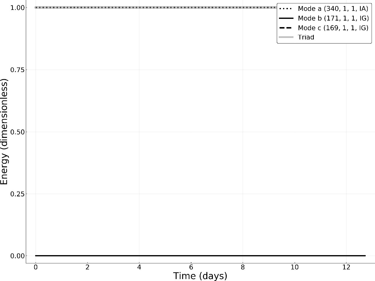
Fig. 3.

Time evolution of the mode quadratic energies associated with the solution of the three-wave interaction equations (33) for the modes of Triad 3 of Table 2. The present triad is non-resonant.
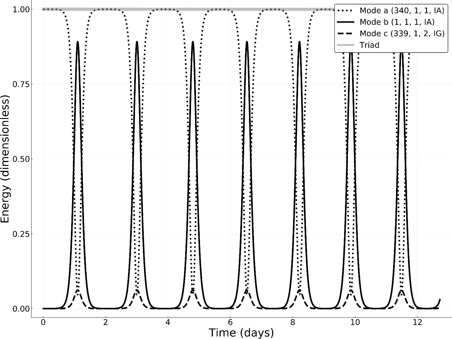
Fig. 4.

Time evolution of the mode quadratic energies associated with the solution of the three-wave interaction equations (33) for the modes of Triad 1 of Table 2. The present triad is nearly resonant.
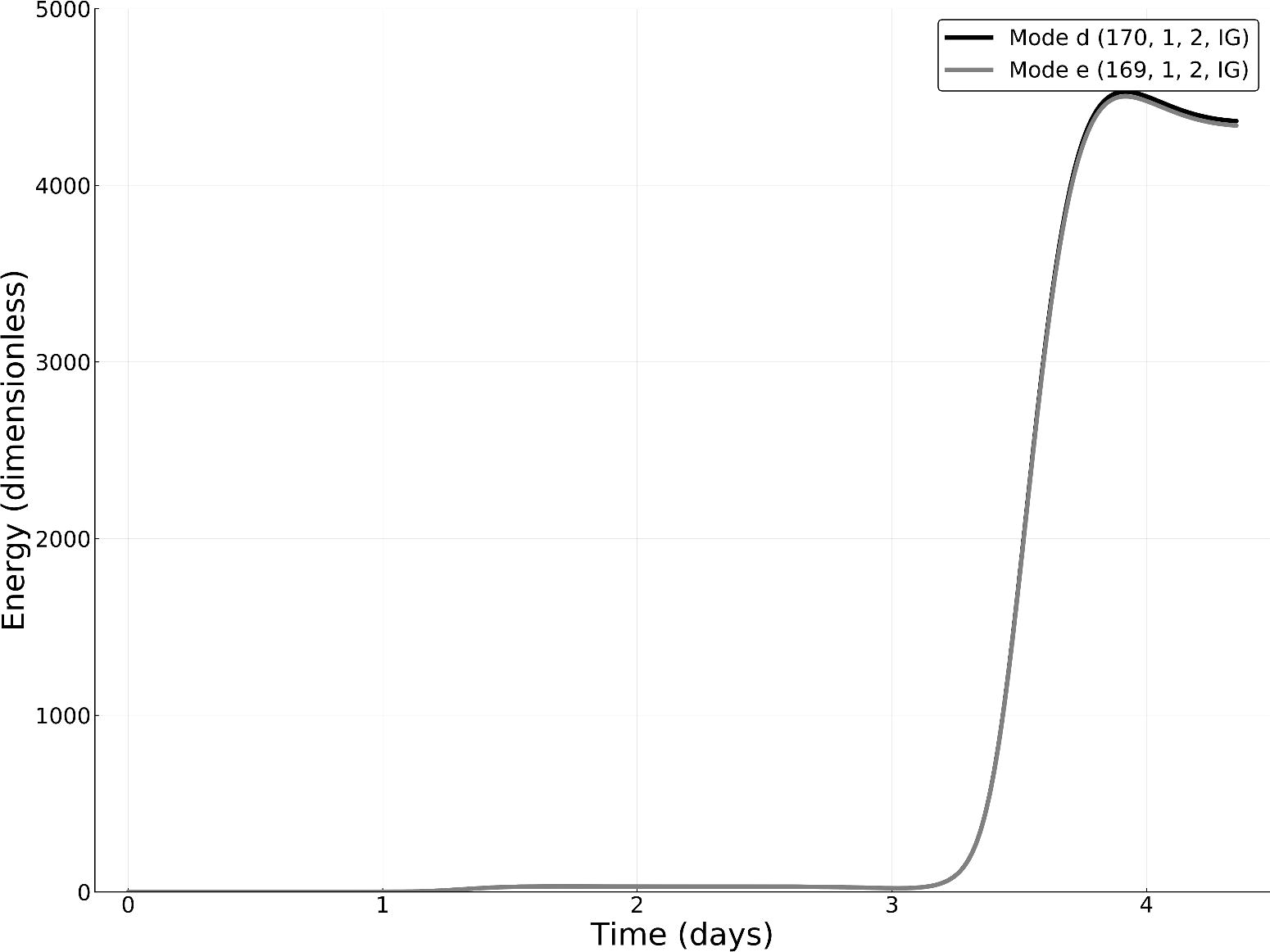
Fig. 5.

Numerical solution of the linearized system (39) composed of modes (170,1,2,IG) and (169,1,2,IG) of Triad 2. These modes are parametrically forced by the mode (339, 1, 2, IG) of Triad 1. This solution presents a maximal Lyapunov exponent λL=1.35×10⁵s1.
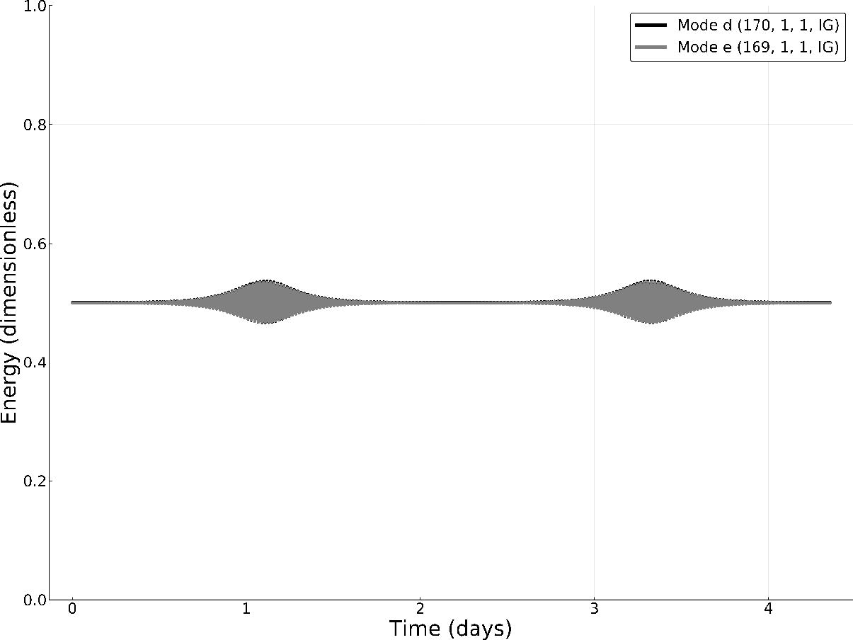
Fig. 6.

Numerical solution of the linearized system (39) composed of modes (170,1,1,IG) and (169,1,1,IG) of Triad 13. These modes are parametrically forced by the mode (339, 1, 2, IG) of Triad 1. This solution presents a maximal Lyapunov exponent λL=4.85×10¹⁰s1.
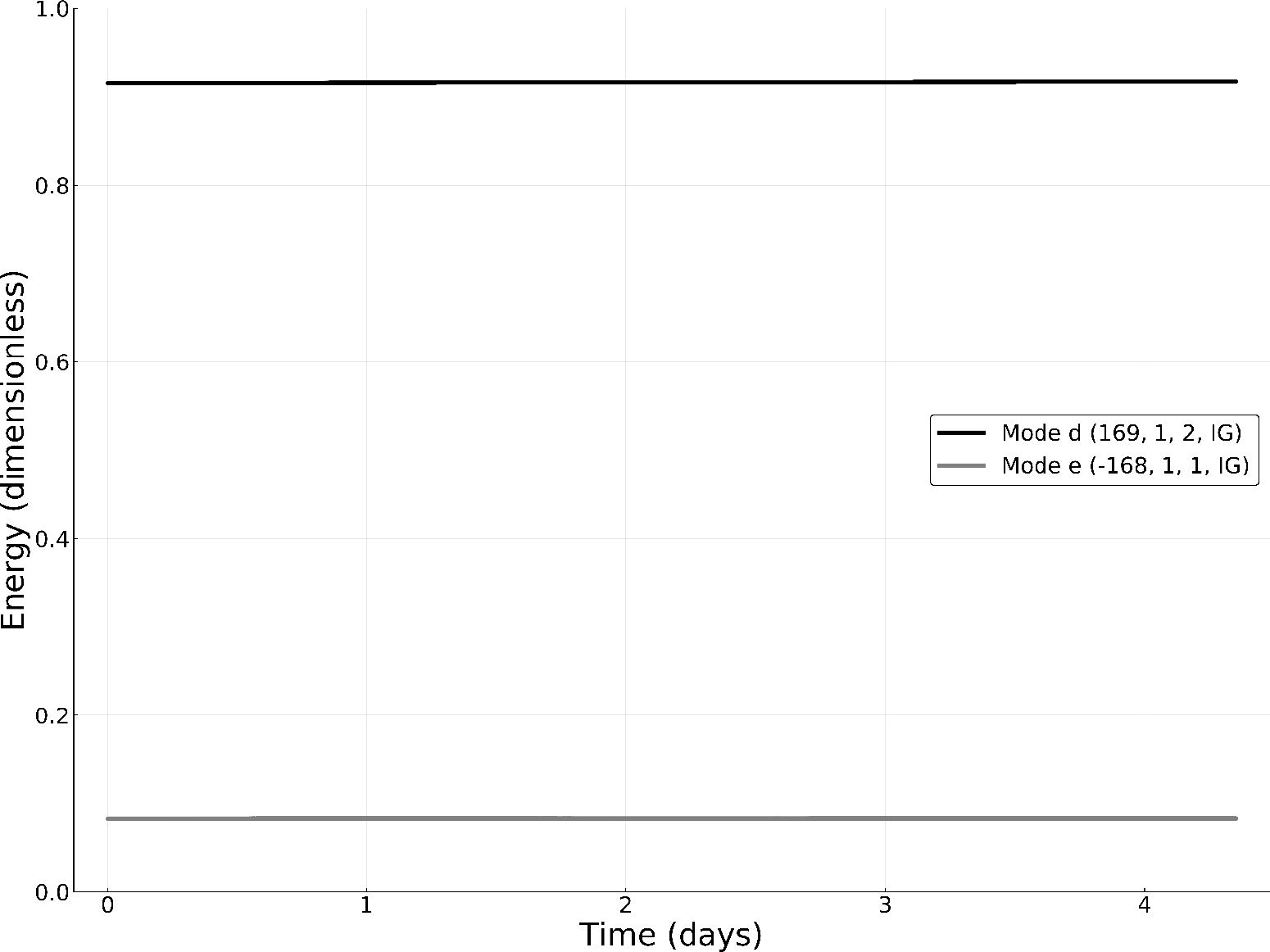
Fig. 7.

Numerical solution of the linearized system (39) composed of modes (169,1,2,IG) and (–168,1,1,IG) of Triad 15. These modes are parametrically forced by the mode (1, 1, 1, IA) of Triad 1. This solution presents a maximal Lyapunov exponent λL=6.59×10¹¹s1.
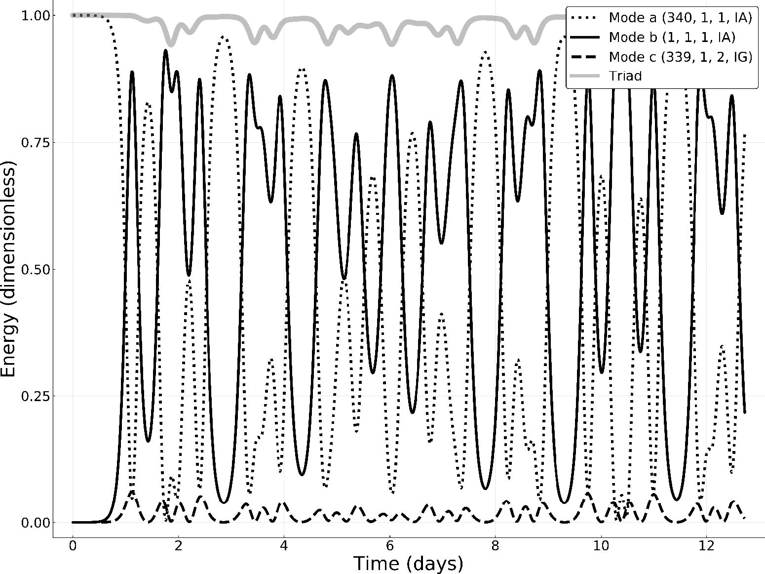
Fig. 8.

Numerical solution of the five-wave system (38) composed of the modes of Triads 1 and 2 of Table 2. This figure illustrates the time evolution of the quadratic energies corresponding to Modes of Triad 1 only.
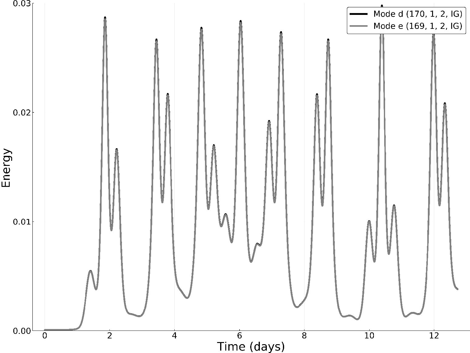
Fig. 9.

This is same as Fig. 8, but illustrating the quadratic energies of the secondary gravity modes of Triad 2.

Language: English
Page range: 1706705 - 1706705
Published on: Jan 1, 2020
Published by: Stockholm University Press
In partnership with: Paradigm Publishing Services

© 2020 André Seiji Wakate Teruya, Carlos Frederico Mendonça Raupp, published by Stockholm University Press
This work is licensed under the Creative Commons Attribution 4.0 License.