
Table 1.
The length of the simulation in setups with different CO2 concentration, characterized by the logarithm n of the CO2 concentration relative to that of the control run (see Equation (1)).
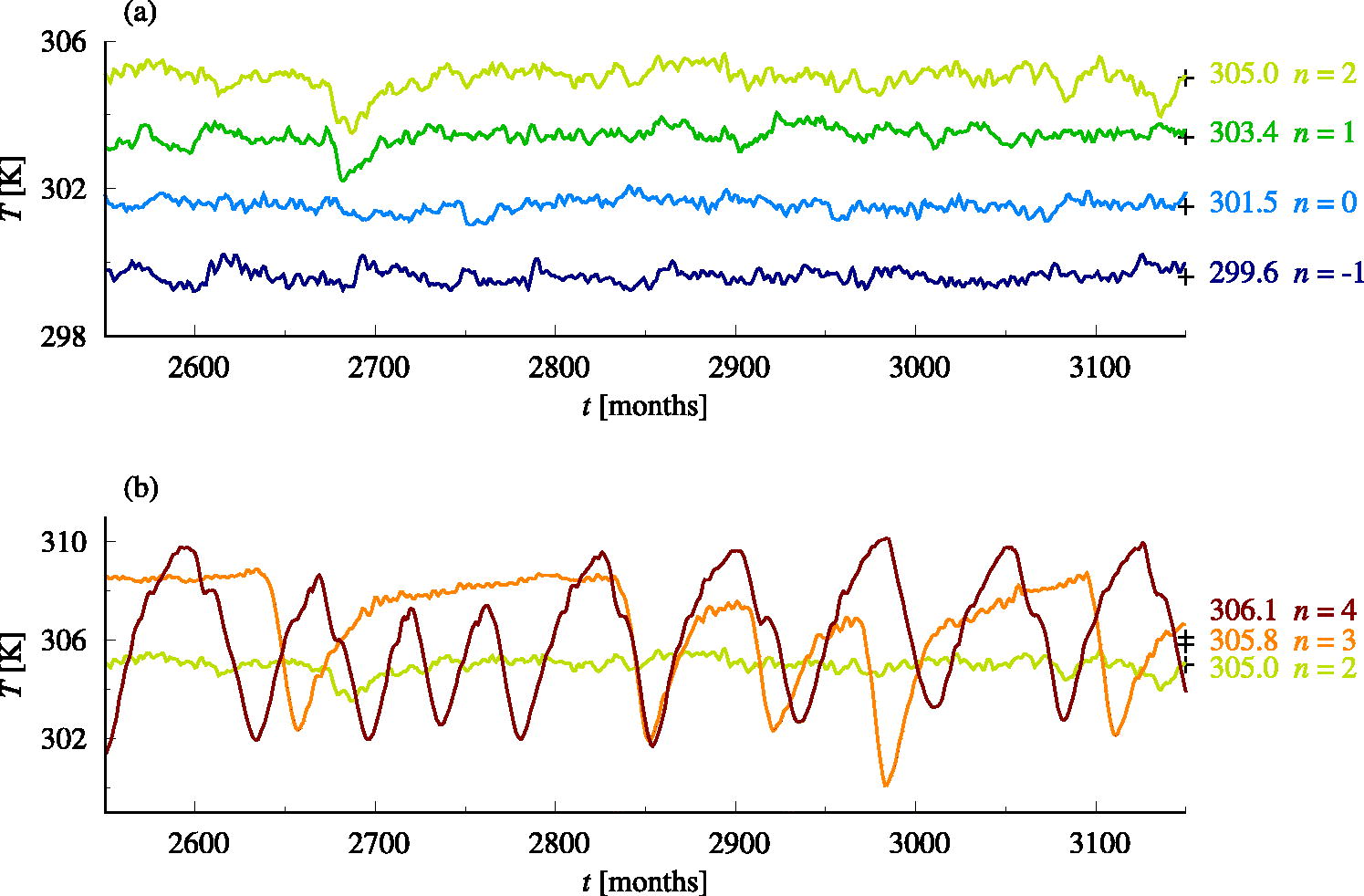
Fig. 1.
The global mean surface temperature as a function of time in setups with different CO2 concentration, labeled by n. The temporal mean is also marked. The setup with n = 2 appears in both panels.
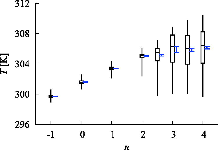
Fig. 2.
Temporal statistics of the global mean surface temperature as a function of the logarithm n of the relative CO2 concentration. Boxes represent the first quartile, the median, and the third quartile in time, and whiskers mark the temporal minimum and maximum. The temporal mean, with an error bar (see text), is included in blue next to the corresponding box.
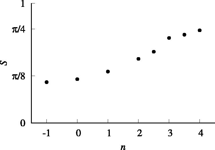
Fig. 3.
The temporal mean of the quantifier S of the characteristic size (see text) as a function of the logarithm n of the relative CO2 concentration.
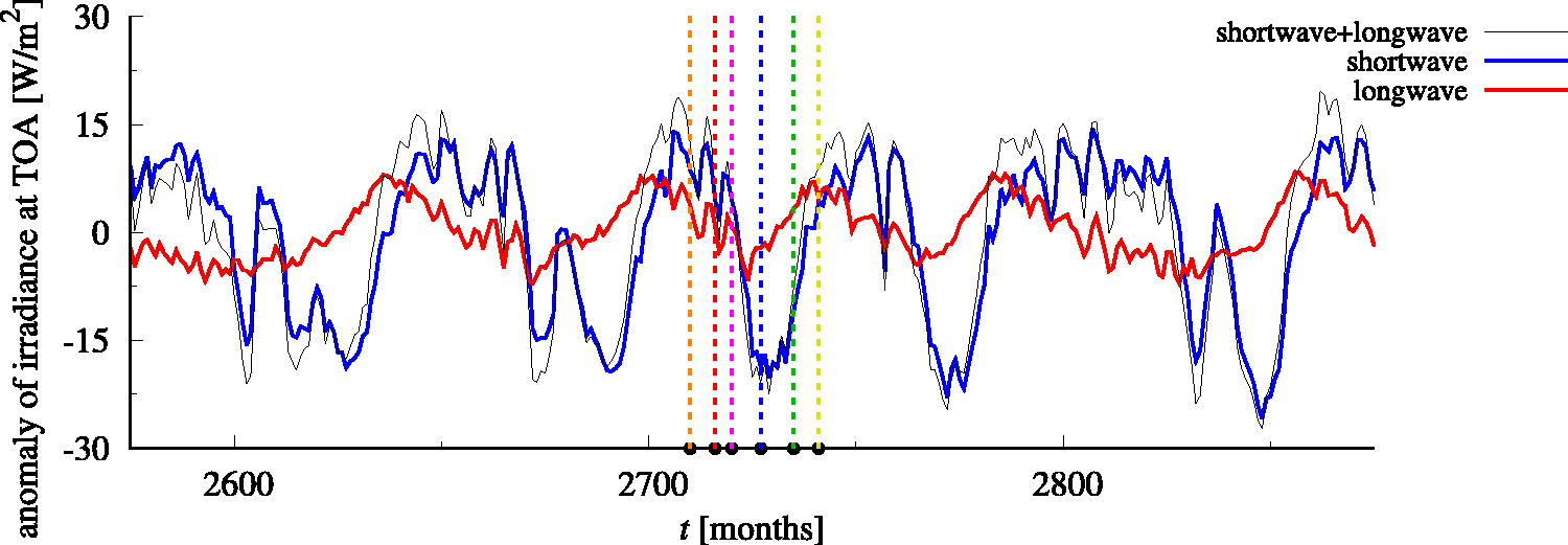
Fig. 4.
Globally averaged irradiance at TOA, as indicated in the legend, after subtracting the temporal mean, as a function of time. The time instants marked by vertical lines with black circles correspond to those of Figs. 6 and 7, and are also used later on. n = 4.
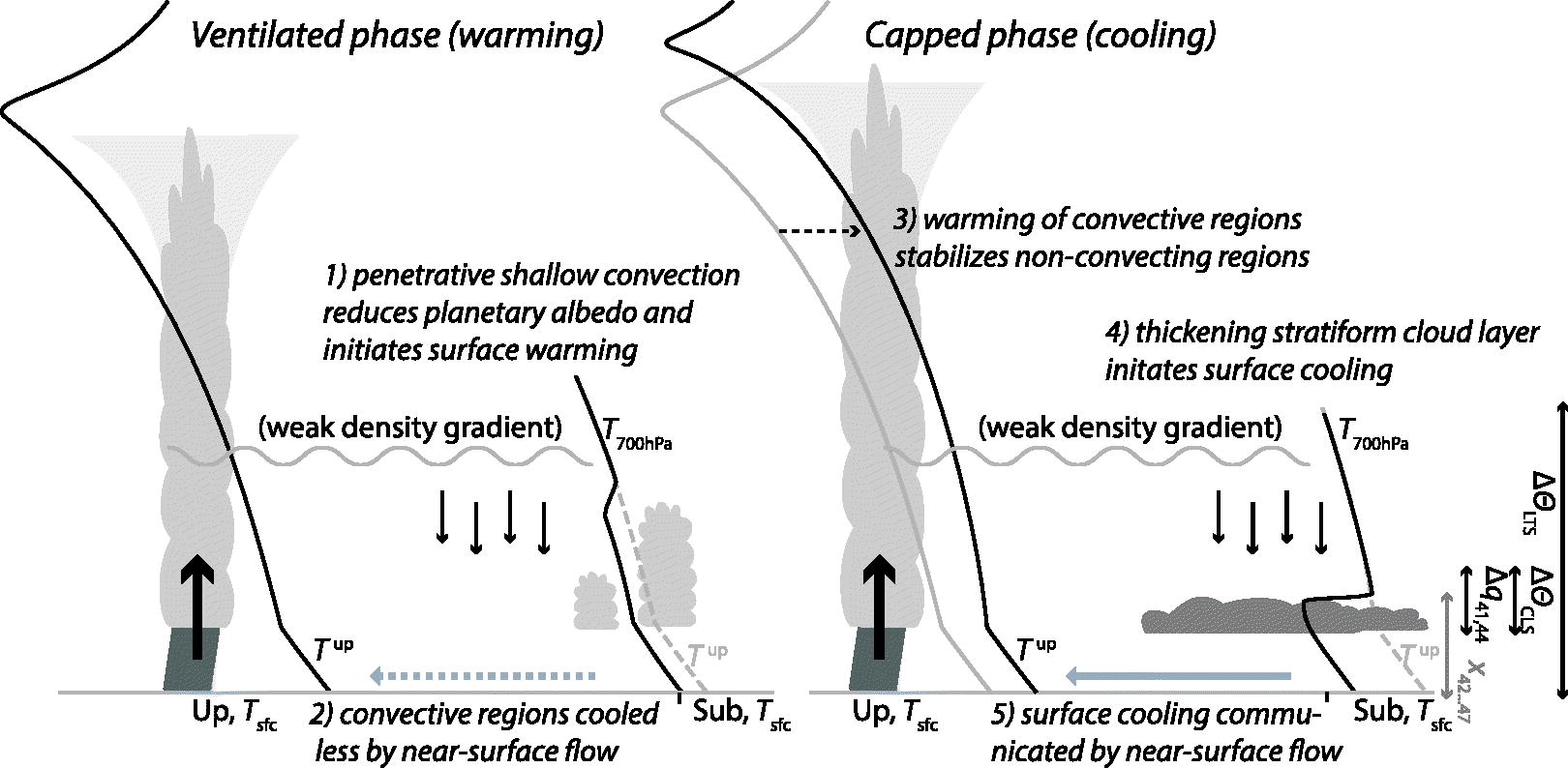
Fig. 5.
Illustration of the cycle between ventilated and capped phases. A key factor for step 3) is the weak density gradient. Since density gradients are attenuated very fast (e.g. Sobel and Bretherton, 2000), the free tropospheric temperature profile of the convective region () is approximately imposed on the subsiding region. Below the free troposphere, the temperature profiles are different, which is illustrated by the difference between the black solid and gray dashed lines in the region of subsidence. These preconditions cause stability variations in the subsiding region that result in variations of the penetrative power of shallow convection. See the main text for more details (Section 4.1 for the labeled quantities).
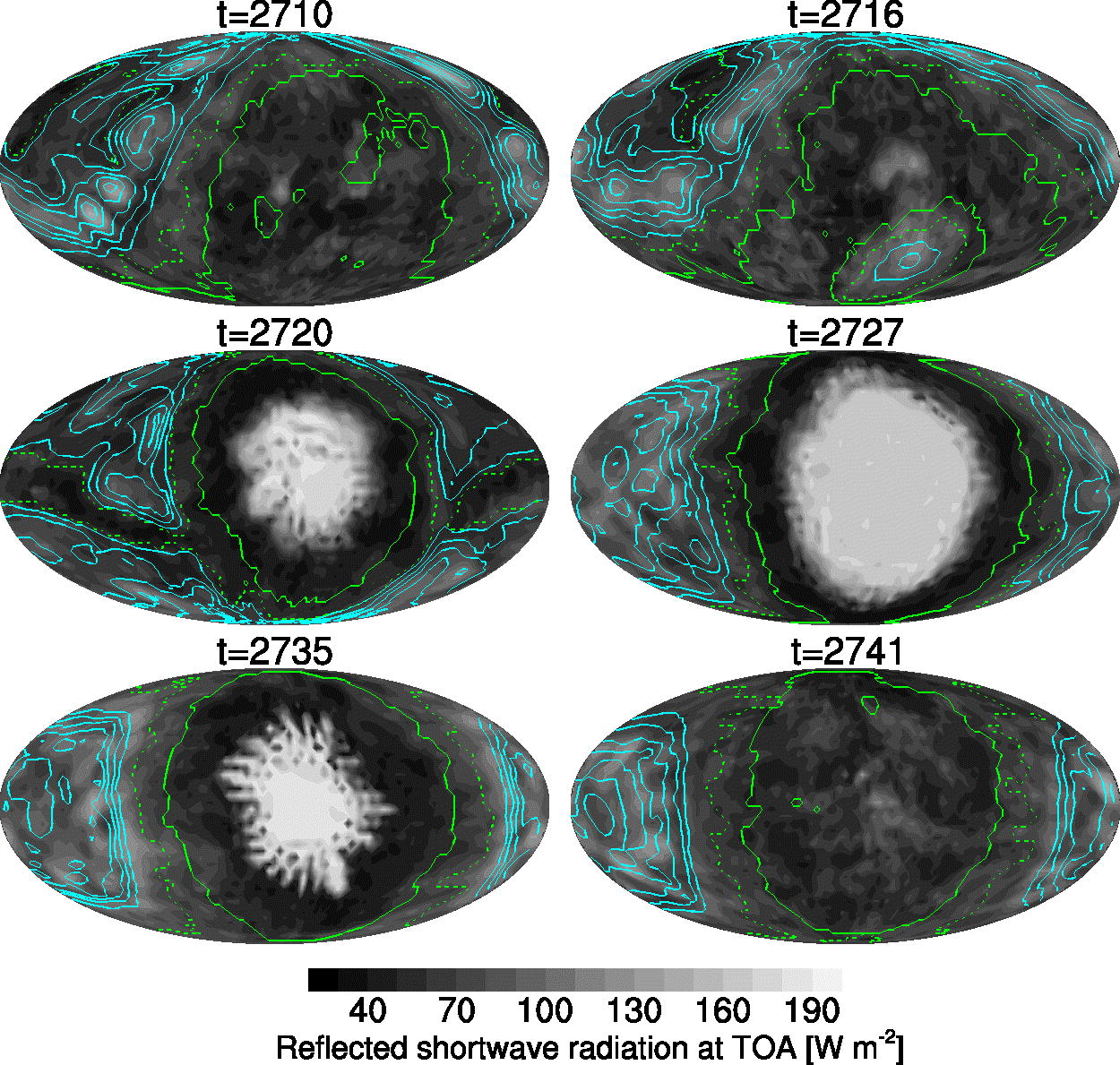
Fig. 6.
Snapshots of upward shortwave irradiance at TOA. The time instants are indicated in the panels and are also marked in Fig. 4. Cyan contour lines denote precipitation in intervals, solid green lines outline the boundary of the dry-subsiding region (ω41 > 0 with at level 41, see also the main text), and green dashed lines demarcate the boundary of the region where ω41 > 0. n = 4.
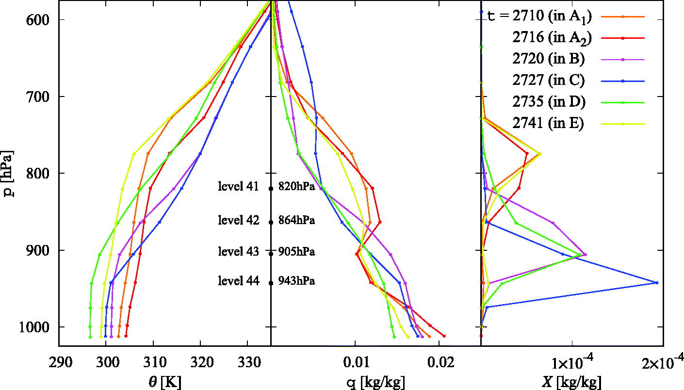
Fig. 7.
Vertical profiles of the potential temperature θ, the specific humidity q, and the cloud liquid water content X, averaged for the dry-subsiding region, at the time instants of Fig. 6 (also marked in Fig. 4) as indicated in the legend. The labeling refers to the sectioning introduced in Fig. 10; sections A and E compose the ventilated phase. Model levels are marked on one vertical axis at the corresponding pressure coordinate averaged spatially (over the dry-subsiding region) and temporally. n = 4.
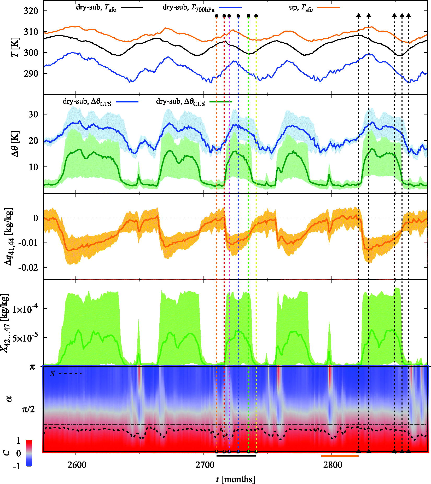
Fig. 8.
The time evolution of several quantities as given on the vertical axis and in the legend; see Table 2. Solid lines mark spatial means, while shaded areas correspond to the interval between the 5th and the 95th spatial percentile. In the uppermost plot, the corresponding spatial region is indicated in the legend; plots below concern the dry-subsiding region. The bottom plot shows the spatial autocorrelation function of ω41 color coded, separately for each time step t, as a function of the angle α of separation. The dashed black line, S, is a measure of size (see Equation (2) and the corresponding explanation), and it is compared to an ideal value (dot-dashed black line) that would correspond to a cosine-shaped autocorrelation function. The vertical lines with circles mark the time instants selected for Figs. 6 and 7, and they also appear, together with the vertical lines with triangles, in Figs. 10–11. The black and orange line segments next to the horizontal axis correspond to time intervals with a major and a minor cooling event, and are highlighted in Figs. 10–11. n = 4.
Table 2.
The quantities most relevant for the cooling dynamics.
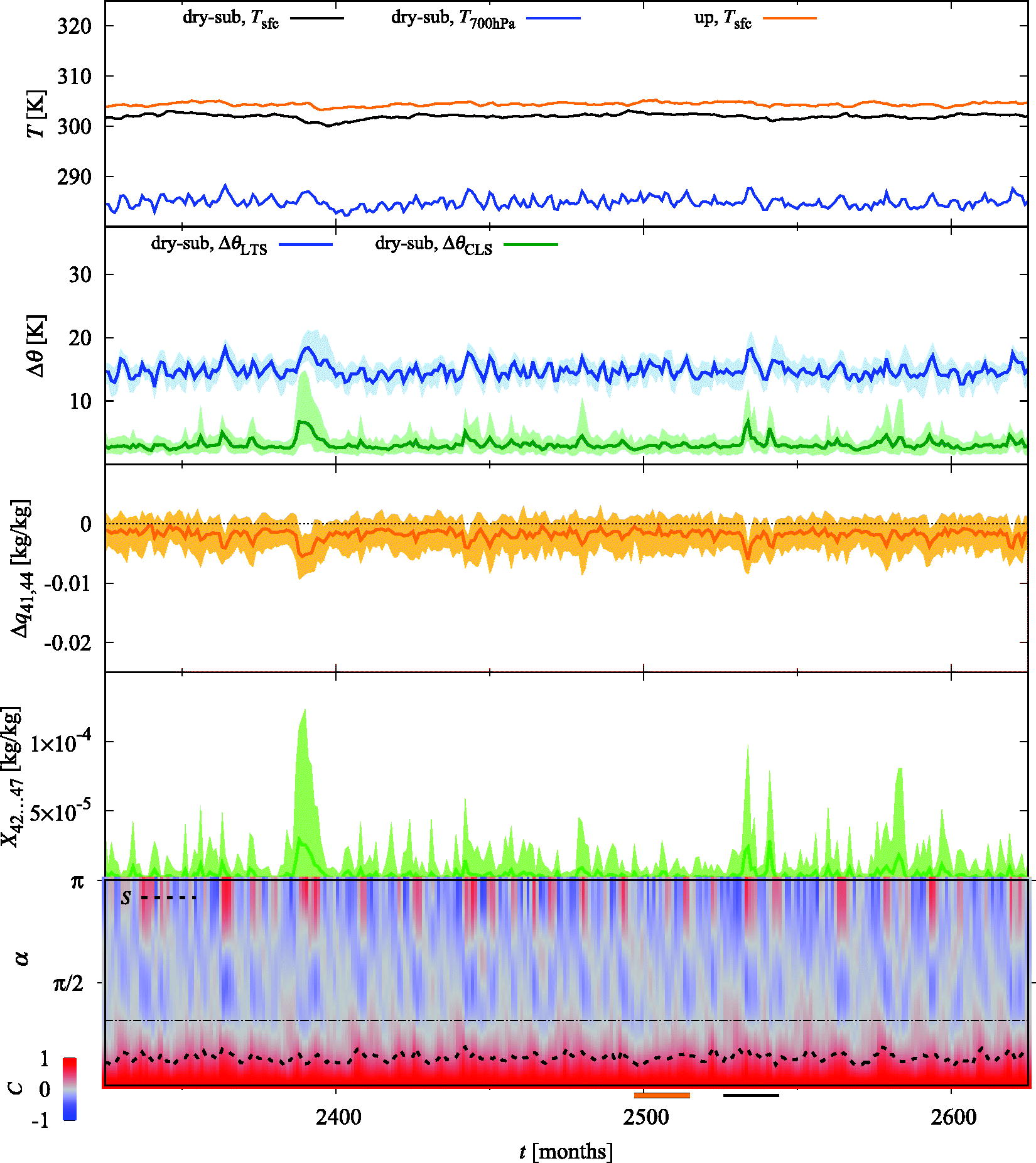
Fig. 9.
Same as Fig. 8 for n = 1.
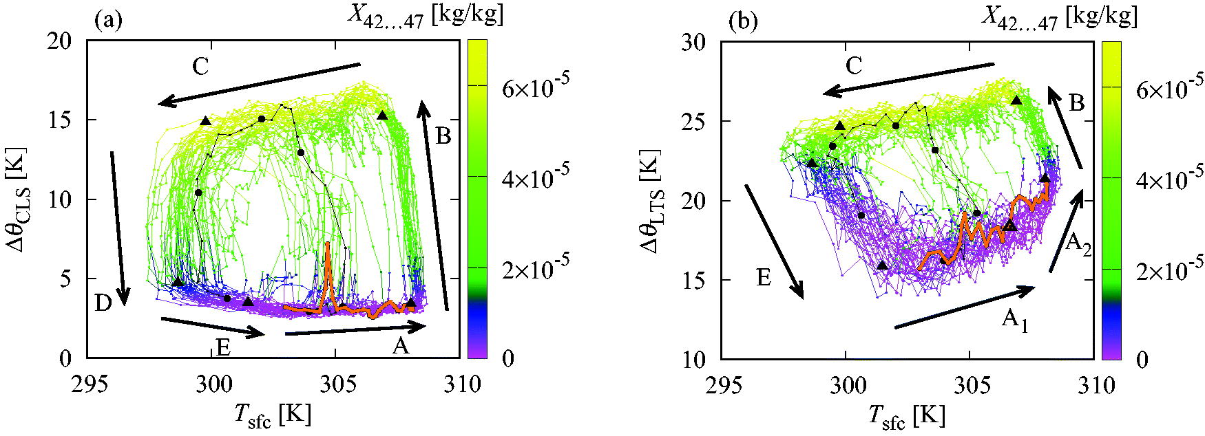
Fig. 10.
Phase space projections for quantities in the dry-subsiding region: the spatial mean of the surface temperature Tsfc, of (a) the cloud-layer stability ΔθCLS and (b) the lower tropospheric stability ΔθLTS, and of the cloud liquid water content All months of the simulation are plotted between t = 2000 and 5000 (to optimize visibility), and consecutive months are linked by a colored line. The labeled arrows indicate the direction of the time evolution, and correspond to separate sections in the dynamics (see text). The time instants marked by circles and filled triangles in Fig. 8 are also marked here in black, with the same symbols. In panel (b), an unfilled triangle is also displayed between the two subsections of section A, corresponding to t = 2809 along the orange trajectory. The time evolution highlighted in black (between the first and the last circle) and in orange (before the first triangle) corresponds to a major and a minor cooling event, respectively (see also in Fig. 8). n = 4.
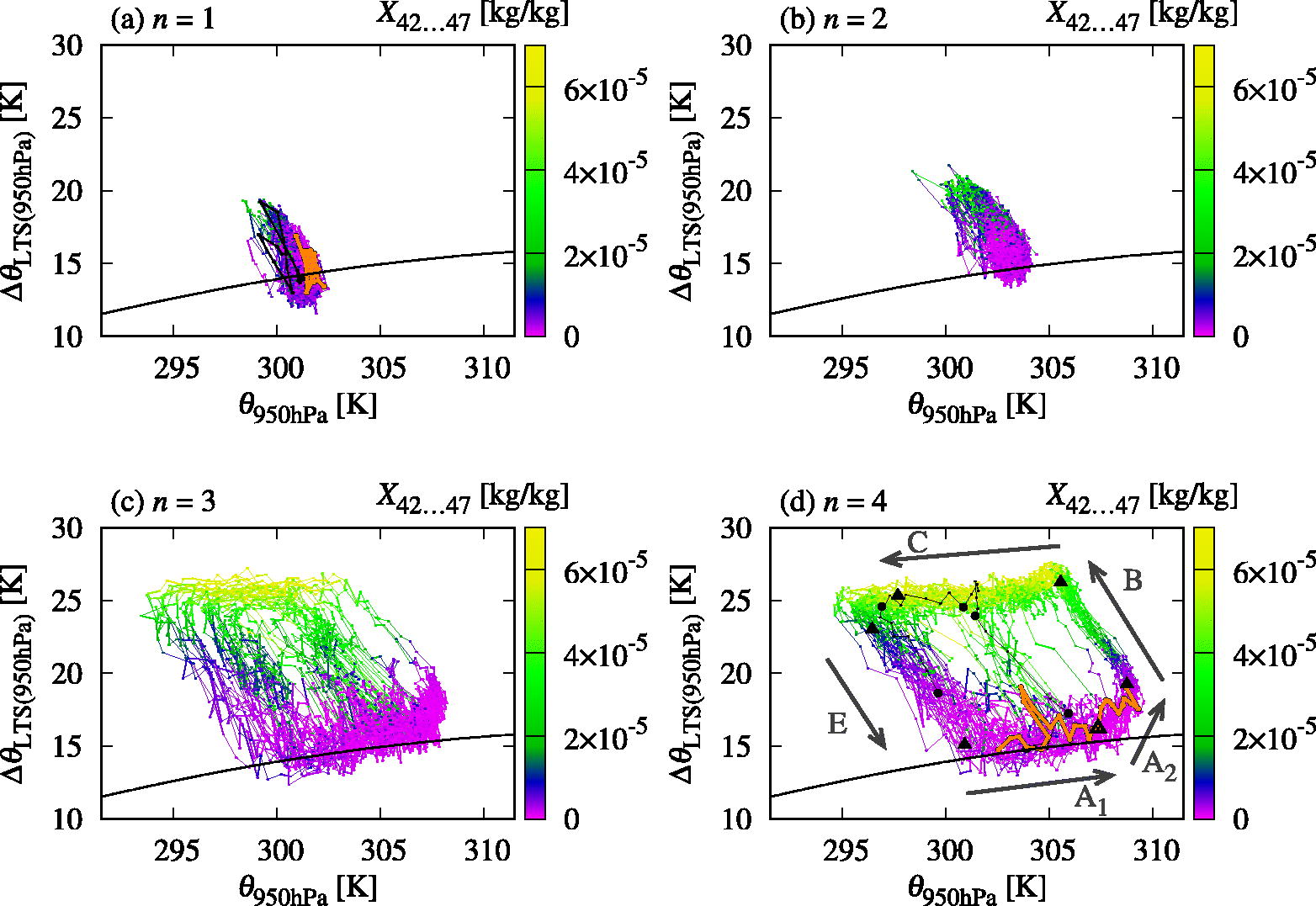
Fig. 11.
Phase space projection: the spatial mean of the near-surface potential temperature θ950hPa, the lower tropospheric stability Δθ, and the cloud liquid water content in the dry-subsiding region. Additional features are marked as in Fig. 10b. Furthermore, Δθ implied by the moist adiabat at given θ950hPa (Bony et al., 2016) is indicated as a black line. Note that the actual stratification is not set by this adiabat, see the main text for more detail. The different panels concern setups with different CO2 concentration, as indicated.