
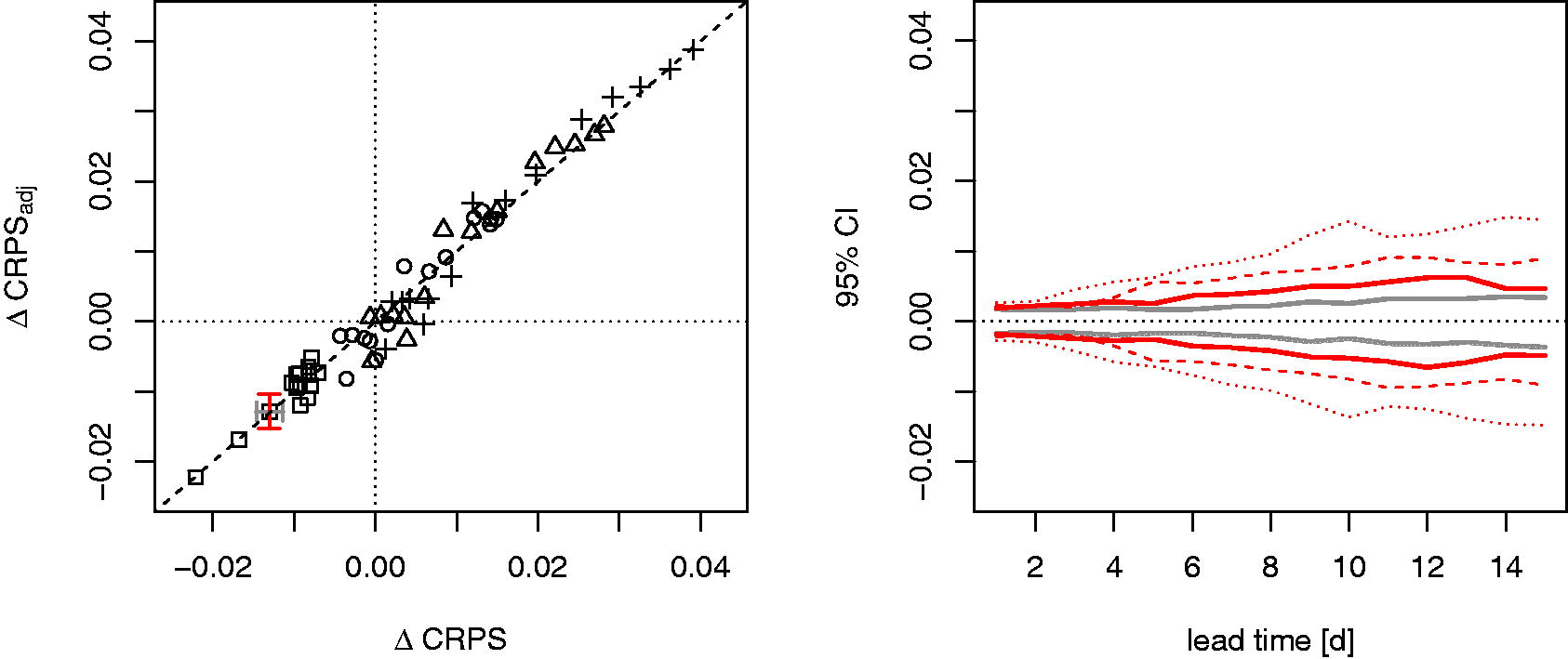
Fig. 1.
Left: comparison of scores computed from actual (p, q) ensembles () and adjusted scores based on a (8) subset of members (). The scores plotted here are CRPS normalised differences between the (0,50) reference ensemble and the baseline multi-model combinations (40,40), (20,120), (10,160), and (200,0) as represented by squares, circles, triangles, and crosses, respectively. Each symbol corresponds to the result for one lead-time ranging between 1 and 15 days. Right: amplitude of the confidence intervals (CI) associated with the CRPS normalised differences (grey line) and the adjusted CRPS normalised differences (red lines) based on (2, 4), and (8) subsets of members (dotted, dashed, full lines, respectively), as a function of the forecast lead-time. CI are estimated by block-bootstrapping with blocks of three days. Results are shown for the comparison between the (0,50) and the (40,40) ensembles only. CI at day 3 based on a (8) subset of members are reported on the plot on the left. Note that the vertical axes have the same scale in both plots.
Table 1.
Gain in experiment computational time and accuracy of the score estimates based on adjusted scores for different sizes of ensemble subset.
Table 2.
Same as Table 1 but for score estimates based on different verification sample sizes and using the actual complete ensemble with p Lres and q Hres members.
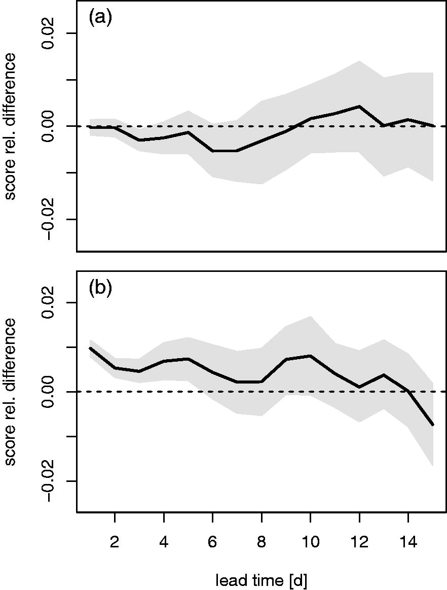
Fig. 2.
Relative difference between CRPS and adjusted CRPS for a (40,40) ensemble as a function of the forecast lead time. The score adjustments are based on a (2) ensemble subset. Generalised multi-model exchangeability conditions are respected in (a) and violated in (b). Mean difference over the verification period (black curve) and variability as measured by block-bootstrap 90% confidence intervals (grey plume).
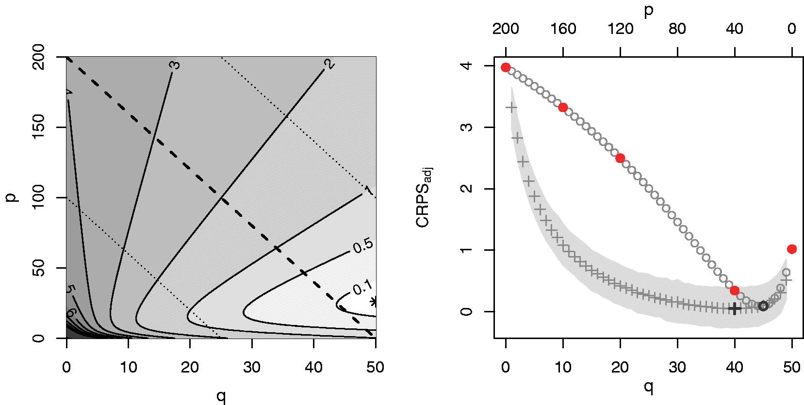
Fig. 3.
Left: ensemble-adjusted CRPS of a dual-resolution ensemble as a function of the number of Lres (p) and Hres (q) members combined with equal weighting. The CRPS values are normalised in order to indicate the percentage degradation with respect to the optimal solution among the tested combinations (as indicated by a *). Black lines indicate ensemble combinations with equal performance. The diagonal dashed line indicates ensemble combinations with computational cost equivalent to the (0,50) reference forecast. Dotted lines indicate results for ensemble combinations with half or double the reference computer resources. Right: ensemble-adjusted CRPS () after normalisation as a function of the number of Hres (Lres) members q (p) considering a fixed computational cost equivalent to running 50 Hres forecasts. The plot shows performance for ensembles with equal weighting () and optimal weighting (+) for each combination. Weights are estimated based on a (8) ensemble. Grey shading indicates 90%-confidence intervals (see text). Optima are highlighted in bold. Results for the baseline/reference combinations of the original analysis are indicated in red. Results are valid for 2 m temperature forecast at day 5.
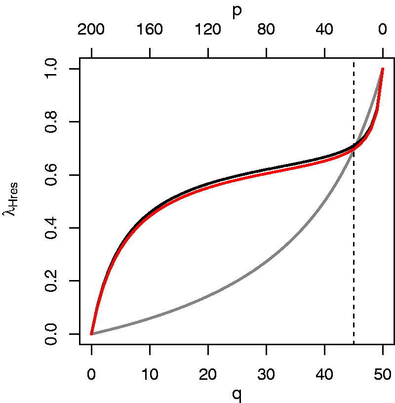
Fig. 4.
Weight associated with the Hres model as a function of the number of Hres (Lres) members q (p) considering a fixed computational cost equivalent to running 50 Hres forecasts: weights when ensemble pooling is applied (grey line), optimal weights estimated from a (200,50) ensemble (black line), optimal weights estimated from a (8) ensemble (red line). The vertical dotted line indicates the optimal (p,q) combination as seen in Fig. 3 (right panel).