Have a personal or library account? Click to login
Physical retrieval of sea-surface temperature from INSAT-3D imager observations Cover

Physical retrieval of sea-surface temperature from INSAT-3D imager observations

By:  and    
Open Access
|Jan 2019

Figures & Tables

Table 1. INSAT-3D imager channel characteristics (Singh et al., 2016a).
Channel numberChannel wavelength (μm)DescriptionPurposeSpatial resolution (km)10.55–0.75VisibleClouds, surface features1.021.55–1.70Short–wave infraredSnow, ice and water phase in clouds1.033.80–4.00Medium–wave infraredClouds, Fog, Fire4.046.50–7.10Water vapourUpper troposphere water vapour8.0510.30–11.30Long-wave infrared windowCloud top and surface temperature4.0611.50–12.50Long-wave infrared windowLower-tropospheric moisture4.0
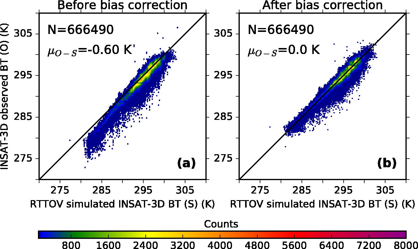
Fig. 1.

Two-dimensional colour histogram plots of the RTTOV simulated and observed INSAT-3D brightness temperature of TIR1 channel, (a) before bias correction and (b) after bias correction.
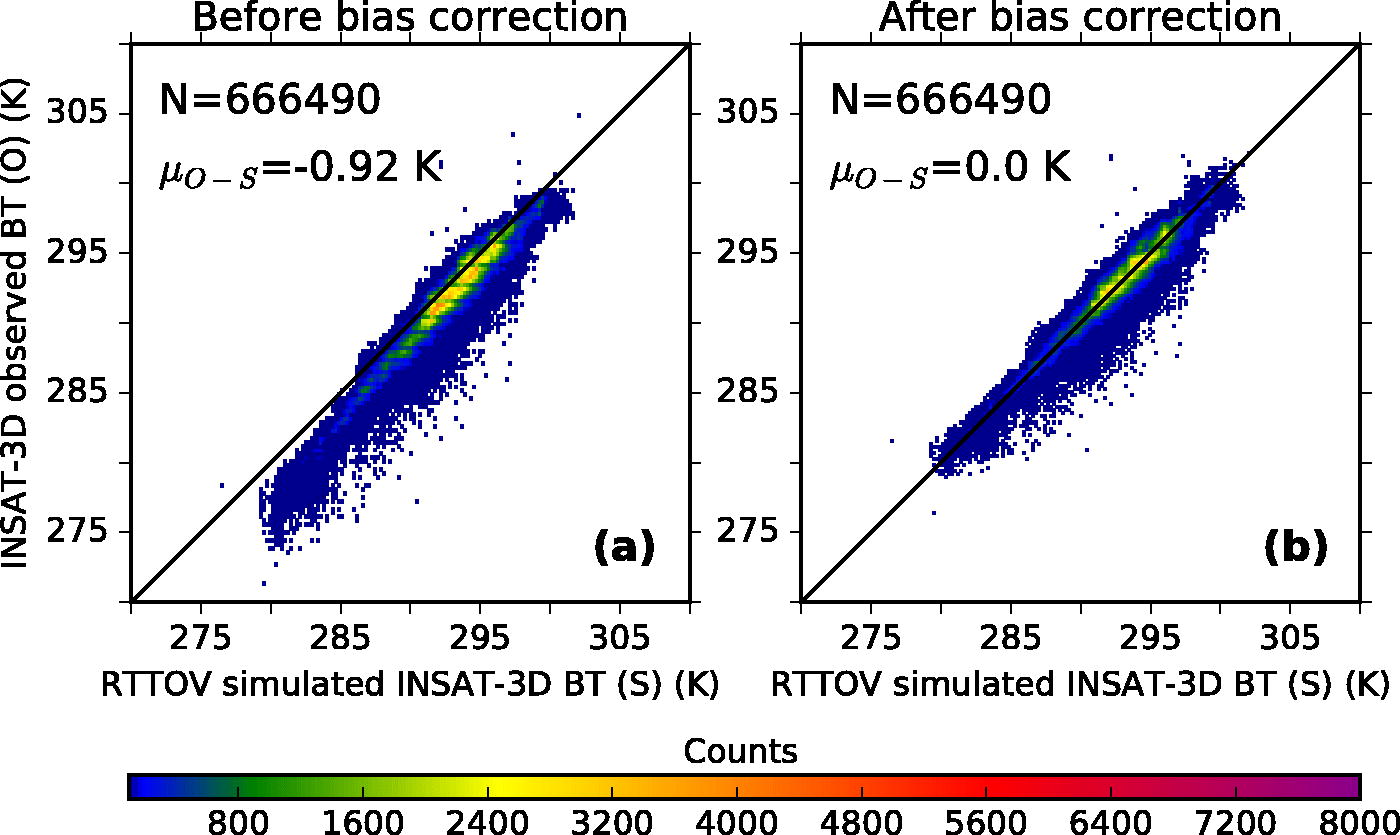
Fig. 2.

Two-dimensional colour histogram plots of the RTTOV simulated and observed INSAT-3D brightness temperature of TIR2 channel, (a) before bias correction and (b) after bias correction.
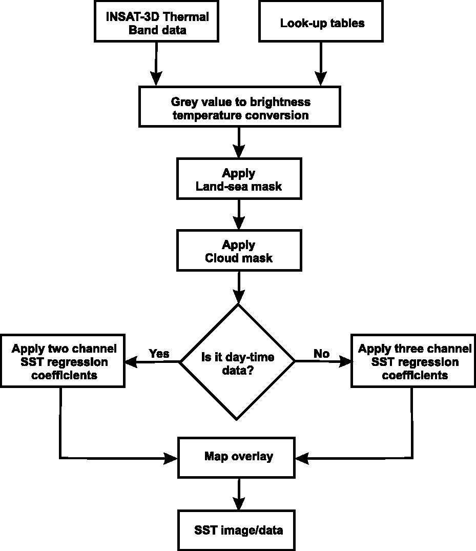
Fig. 3.

Various steps of the operational INSAT-3D SST retrieval algorithm.
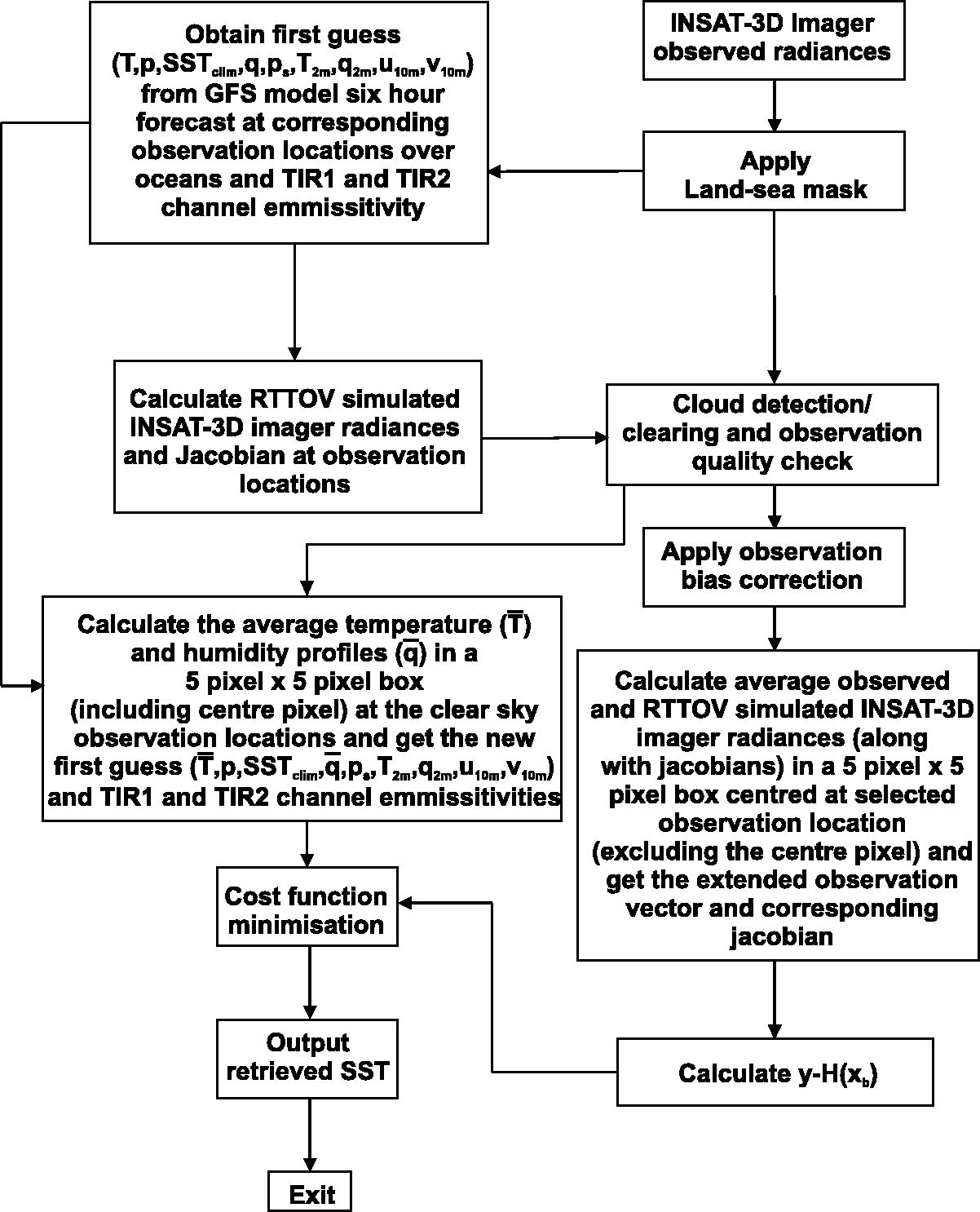
Fig. 4.

Various steps of the OEM fsvis SST retrieval algorithm used for INSAT-3D.
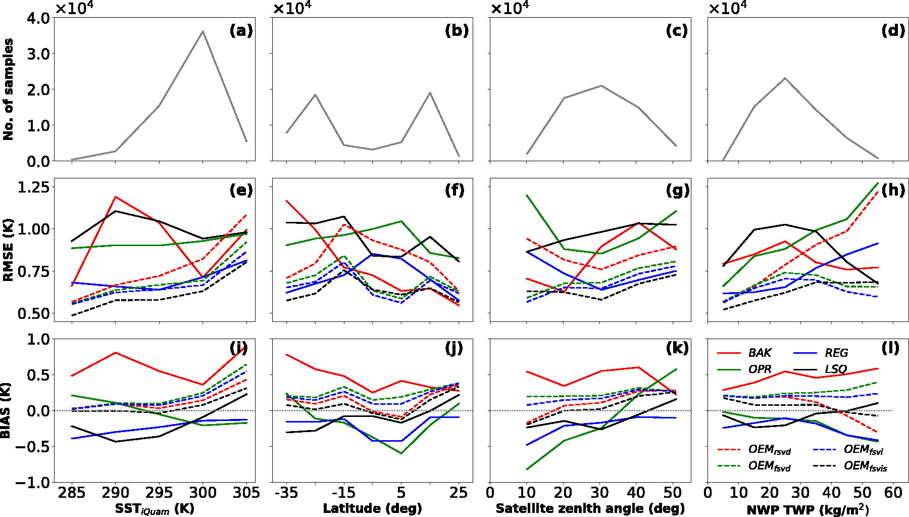
Fig. 5.

Variation of the SST bias and RMSE with respect to (a) iQuam SST, (b) latitude, (c) satellite zenith angle and (d) TCWV.

Table 2.

List of all the SST retrieval algorithms used in this study.

AlgorithmsState vector used,
reduced (R) or full (F)Solution method,
direct (D) or iterative (I)Smoothing applied (Y/N)REG––NOEM rsvd RDNLSQFDNOEM fsvd FDNOEM fsvi FINOEM fsvis FIY

[i] The algorithms are arranged in order of increasing complexity.

Table 3.

Overall validation statistics of the INSAT-3D imager SST retrievals obtained using OPR, REG, LSQ, OEM rsvd , OEM fsvd , OEM fsvi and OEM fsvis against iQuam SST.
Bias (K)RMSE (K)SD (K)Median (K)MADs (K)SSTretSSTtrue¯DFS¯OPR–0.150.920.91–0.210.89––REG–0.170.700.68–0.190.650.81–LSQ–0.150.980.97–0.150.931.002.00OEM rsvd 0.140.820.810.140.700.691.23OEM fsvd 0.230.710.670.210.630.661.13OEM fsvi 0.190.680.650.160.610.661.13OEM fsvis 0.060.630.630.030.590.891.69BAK0.480.860.710.470.66––

[i] The statistics of the background SST (BAK) used in these algorithms is also presented. This statistics is obtained from eight months data (October 2017–May 2018). A total of 60314 collocated pairs were used in calculating this statistics.

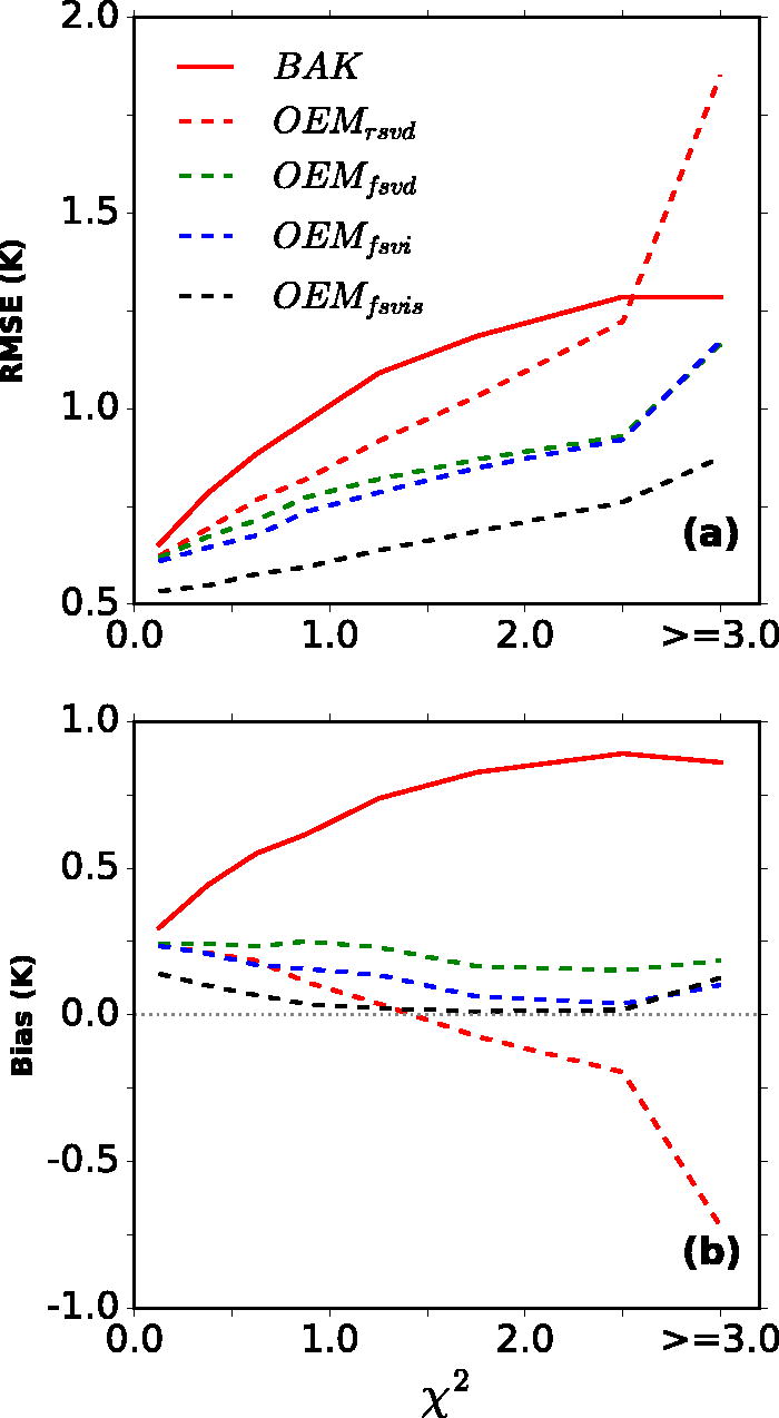
Fig. 6.

RMSE and bias plots of SST retrievals, from different methods, as a function of corresponding χ2 values. Values of the χ2 for the corresponding methods are used for generating these plots. For BAK, χ2 values of OEM rsvd are used.

Table 4.

Validation statistics of the SST retrievals obtained using OPR, REG, LSQ, OEM rsvd , OEM fsvd , OEM fsvi and OEM fsvis against iQuam SST, for day and night separately.
nDay 36796Night 23518Bias (Median)RMSESD (MADs )Bias (Median)RMSESD (MADs )(K)(K)(K)(K)(K)(K)OPR–0.26 (–0.32)0.910.87 (0.84)0.02 (–0.01)0.950.95 (0.92)REG–0.19 (–0.20)0.700.67 (0.64)–0.15 (–0.16)0.710.69 (0.67)LSQ–0.21 (–0.20)1.010.99 (0.95)–0.05 (–0.07)0.930.93 (0.90)OEM rsvd 0.12 (0.10)0.810.80 (0.70)0.17 (0.17)0.840.82 (0.70)OEM fsvd 0.20 (0.17)0.710.68 (0.64)0.29 (0.25)0.710.65 (0.61)OEM fsvi 0.16 (0.14)0.680.66 (0.61)0.24 (0.21)0.680.63 (0.60)OEM fsvis 0.04 (0.0)0.630.63 (0.58)0.01 (0.07)0.640.63 (0.61)BAK0.51 (0.50)0.910.76 (0.72)0.42 (0.43)0.770.64 (0.58)

[i] The statistics of the background SST (BAK) used in these algorithms is also presented. This statistics is obtained from eight months data (October 2017–May 2018).

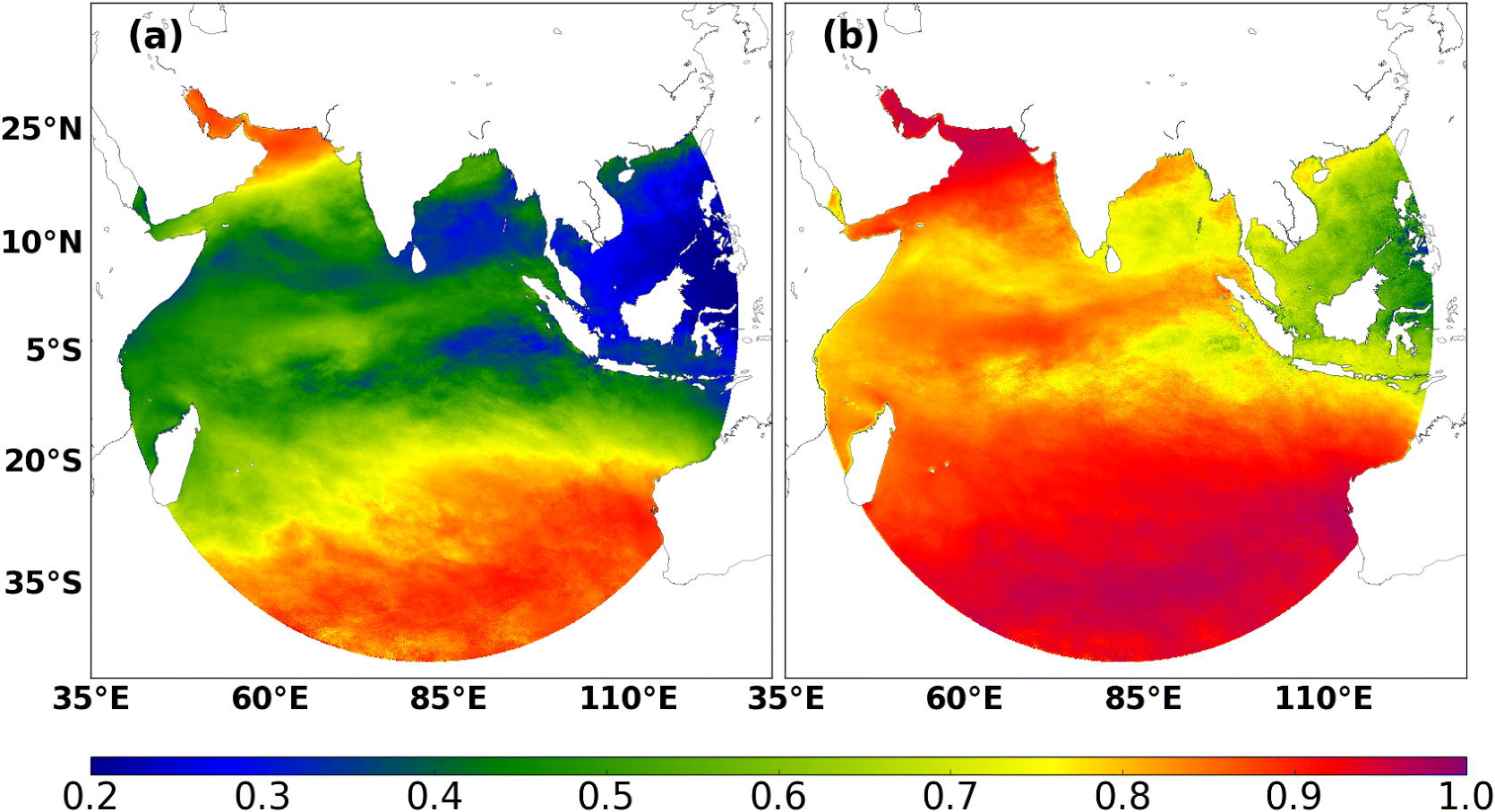
Fig. 7

Spatial maps of the monthly average SST sensitivity, for SST retrieved (a) from OEM fsvi and (b) OEM fsvis , for the month of October 2017.
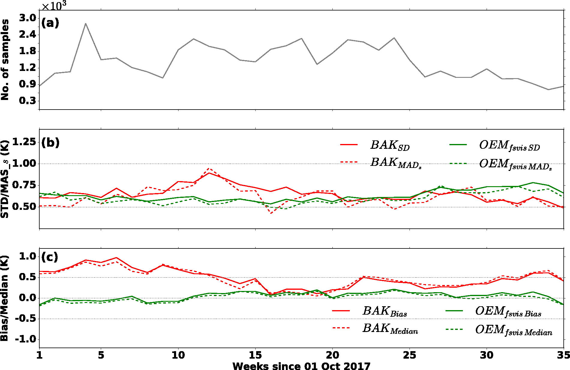
Fig. 8.

Weekly time series of the error statistics, day and night-time combined, of BAK and OEM fsvis SST.
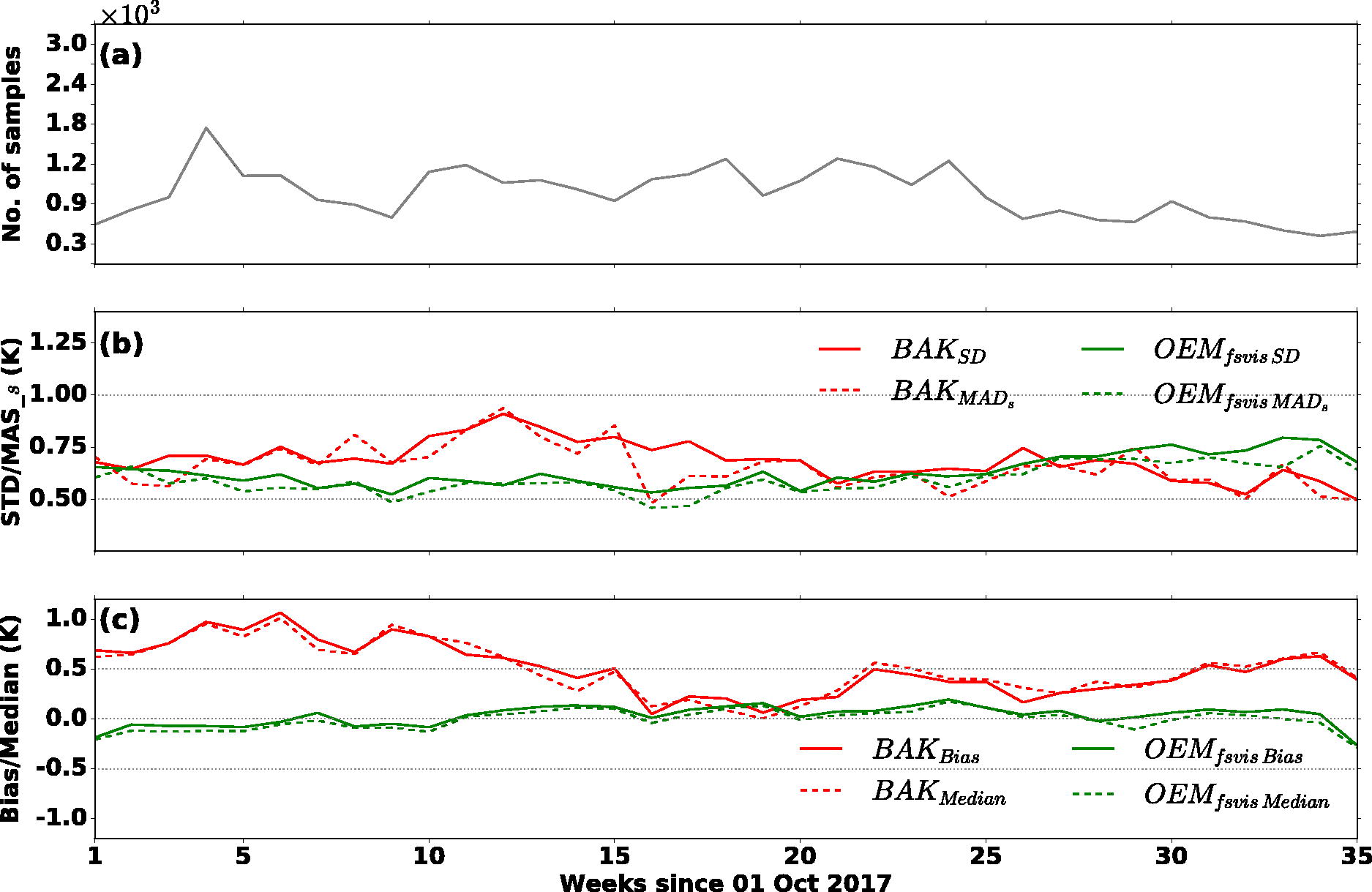
Fig. 9.

Weekly time series of the error statistics, during day-time, of BAK and OEM fsvis SST.
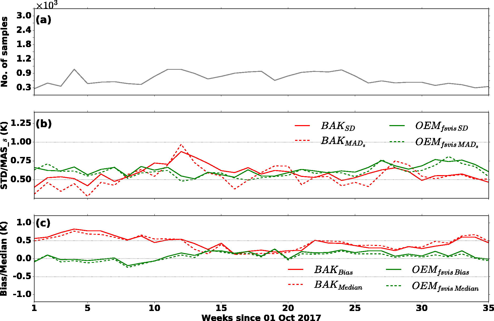
Fig. 10.

Weekly time series of the error statistics, during night-time, of BAK and OEM fsvis SST.
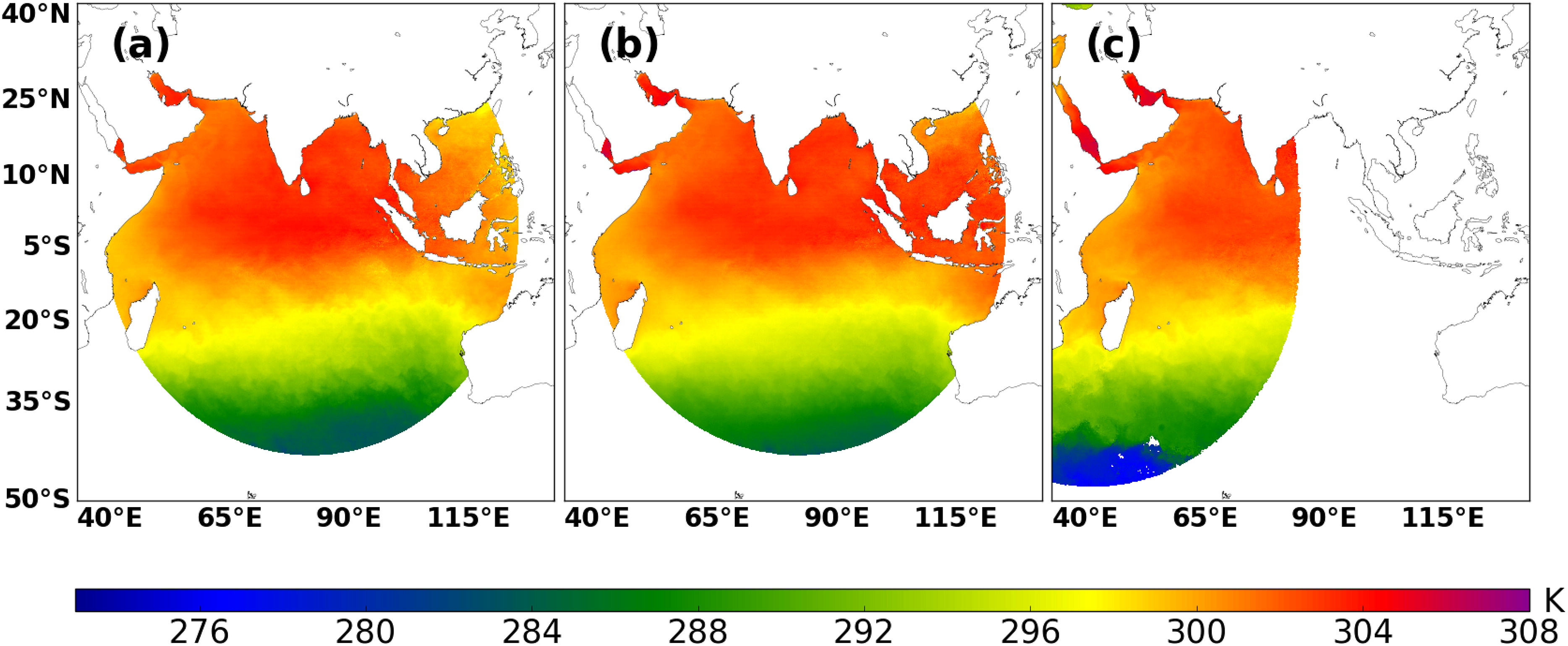
Fig. 11.

Monthly average SST for the month of October 2017. (a) SST retrieved from INSAT-3D observations using REG, (b) SST retrieved from INSAT-3D observations using OEM fsvis and (c) OSI-SAF-SST.
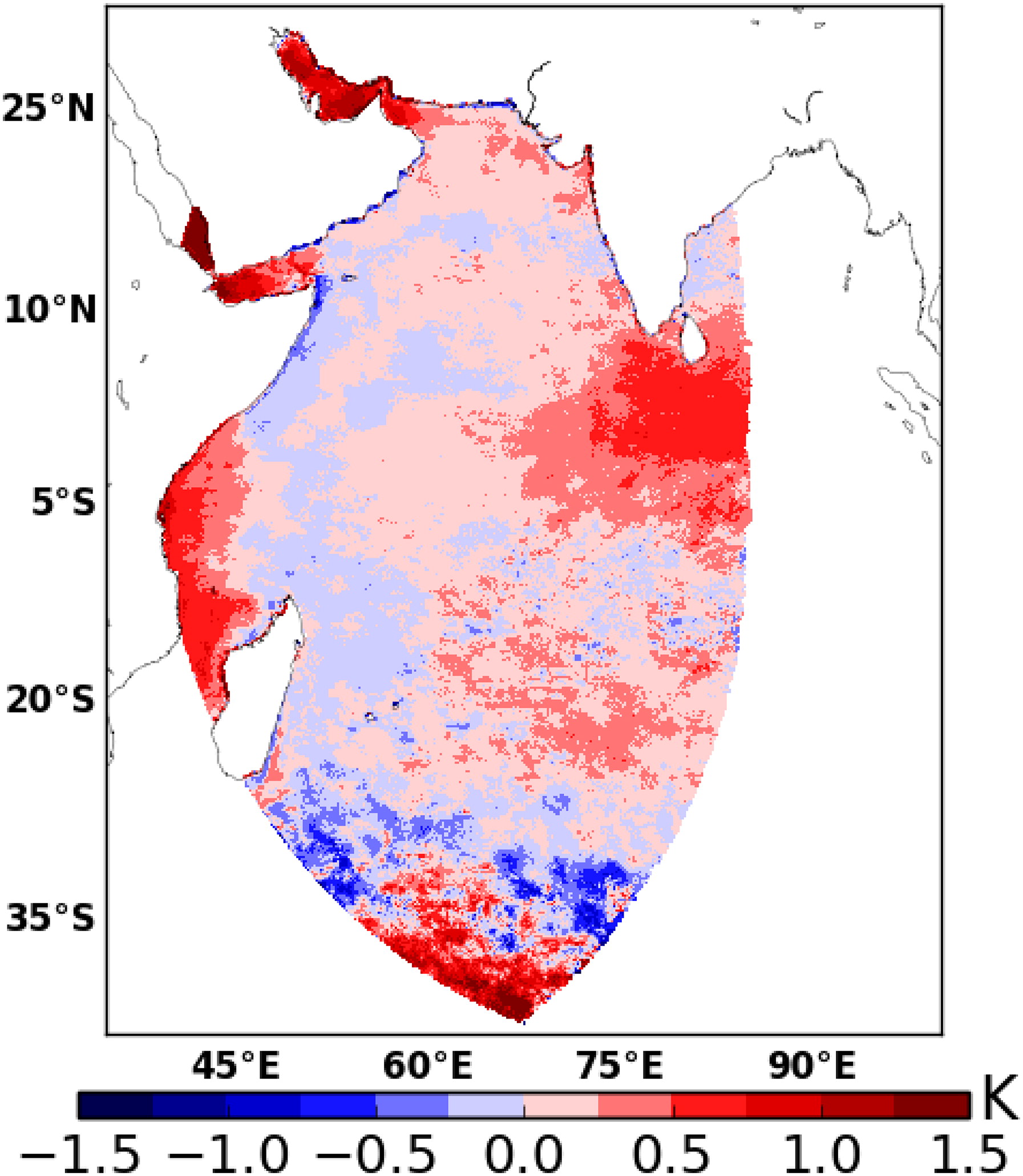
Fig. 12.

Spatial distribution of the improvement parameter, α.

Table 5.

Validation statistics of OEM rsvd , OEM fsvd , OEM fsvi and OEM fsvis calculated for different values of χ2.

Algorithmχ2Bias (K)RMSE (K)SD (K)Median (K)MADs (K)Nχ210.210.680.650.190.6248024 (∼80%)OEM rsvd 1<χ220.00.960.96–0.160.877551 (∼12%)2<χ2–0.431.541.48–0.711.134739 (∼8%)χ210.240.670.620.230.5949731 (∼82%)OEM fsvd 1<χ220.210.840.810.110.777836 (∼13%)2<χ20.170.990.98–0.010.812747 (∼5%)χ210.210.640.600.190.5850925 (∼84%)OEM fsvi 1<χ220.110.800.80–0.020.727005 (∼12%)2<χ20.050.990.99–0.160.752384 (∼4%)χ210.080.560.560.060.5334951 (∼58%)OEM fsvis 1<χ220.020.660.66–0.040.6215856 (∼26%)2<χ20.060.810.81–0.070.809507 (∼16%)

[i] Values of the χ2 for the corresponding methods are used while calculating these statistics.

Language: English
Page range: 1657767 - 1657767
Published on: Jan 1, 2019
Published by: Stockholm University Press
In partnership with: Paradigm Publishing Services

© 2019 Satya P. Ojha, Randhir Singh, published by Stockholm University Press
This work is licensed under the Creative Commons Attribution 4.0 License.