
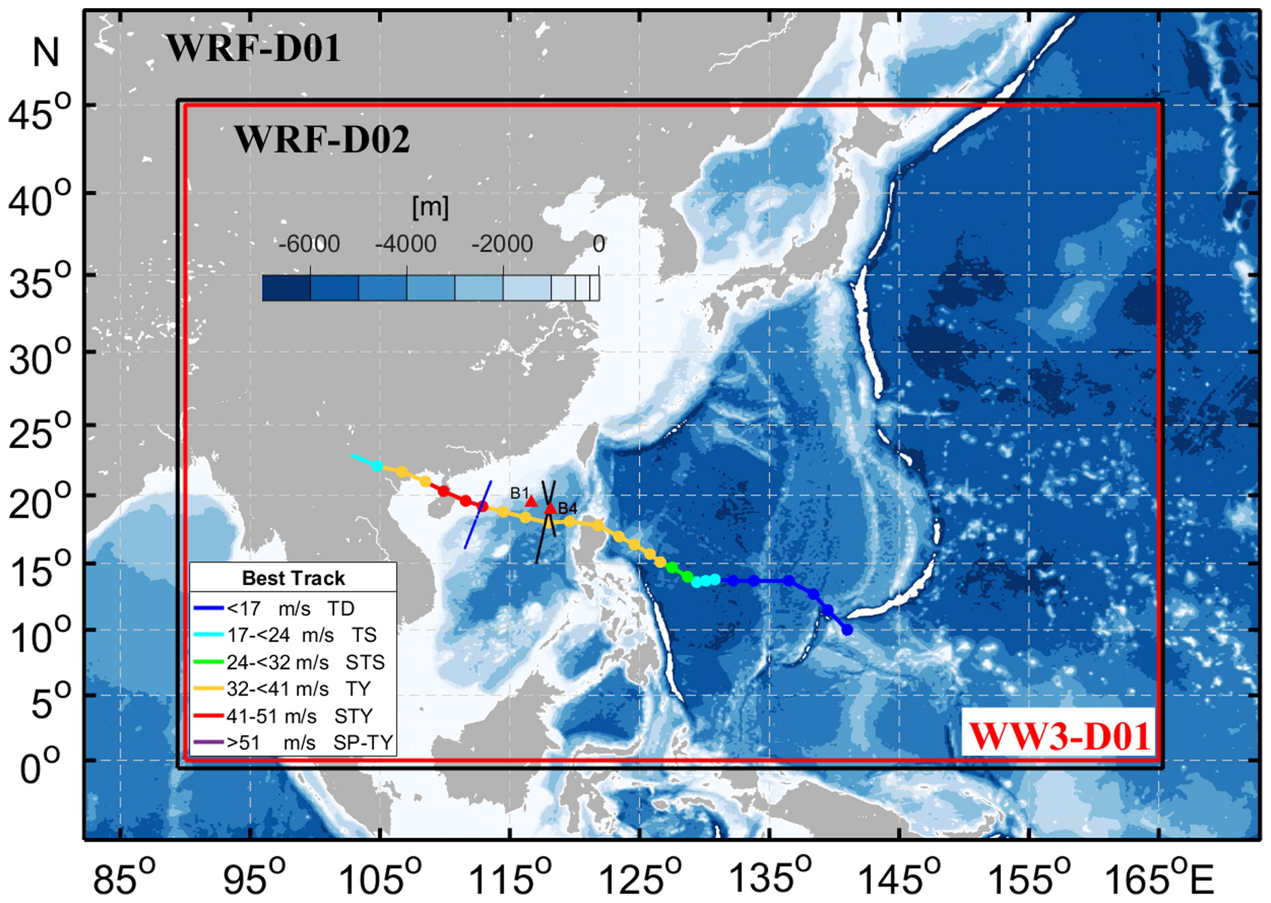
Fig. 1.
Double-layer calculation domains in WRF model (WRF-D01 and WRF-D02), single-layer calculation domain in WW3 model (WW3-D01) and terrain from ETOPO1 (unit: m); Best track and the intensity of severe typhoon Kalmaegi from JTWC, the positions of two buoys (B1 and B4) and scanning paths of SARAL (Janson-2) radar altimeter are marked by coloured dots, red triangles and black (blue) dashed lines, respectively. The intensity is classified into six categories based on maximum 10-m wind speed, i.e., tropical depression (TD), tropical storm (TS), severe tropical storm (STS), typhoon (TY), severe typhoon (STY), and super typhoon (SP-TY).
Table 1.
Summary of altimeter missions and data used in this paper including band-operated, data type, cycle/pass numbers, and data acquisition moment at Kalmaegi’s lifetime, etc.
Table 3.
STD, RMSE and Correlation for , and simulation from different forcing winds at B4.
Table 4.
Same as Table 3, but for B1.
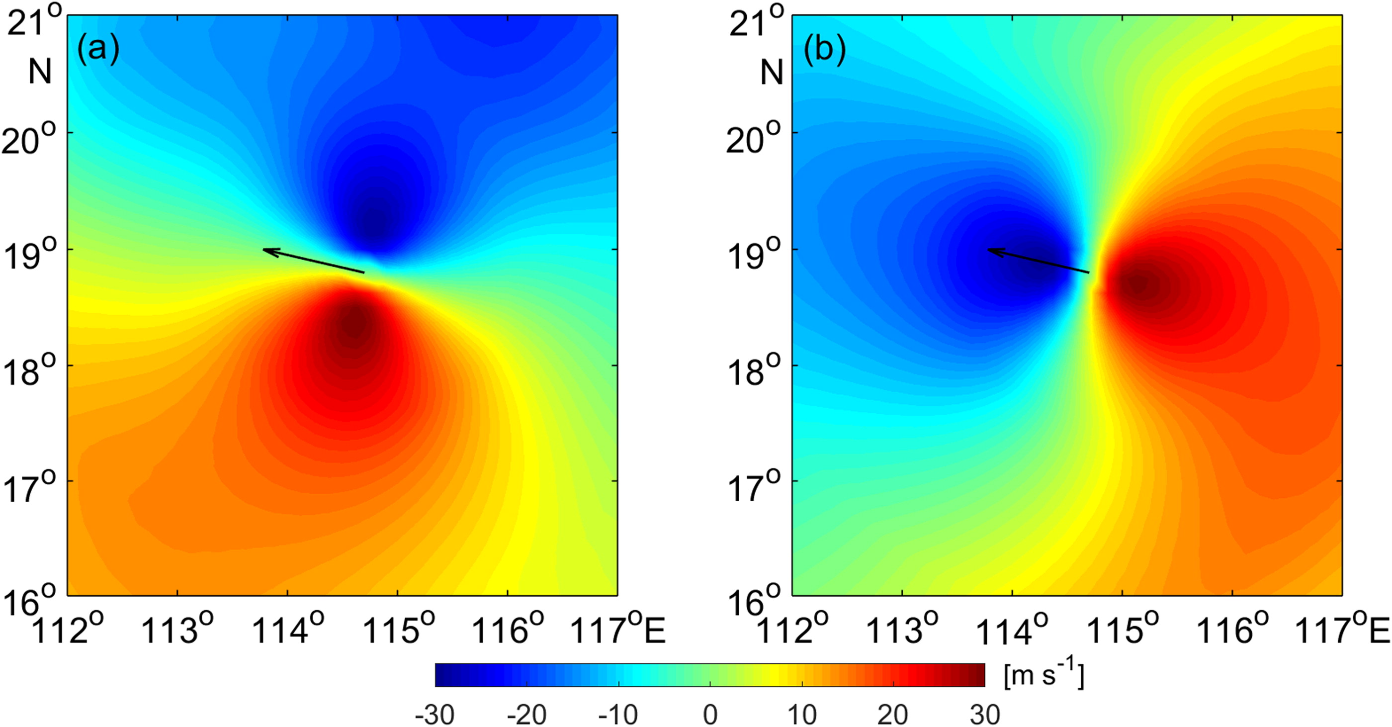
Fig. 2.
Models of H80 of Kalmaegi (1200 UTC 15 Sep). Red and blue areas indicate positive and negative extremes in the velocity field. The left (right) plot is the horizontal (vertical) mode. The black arrow shows the forward speed direction.
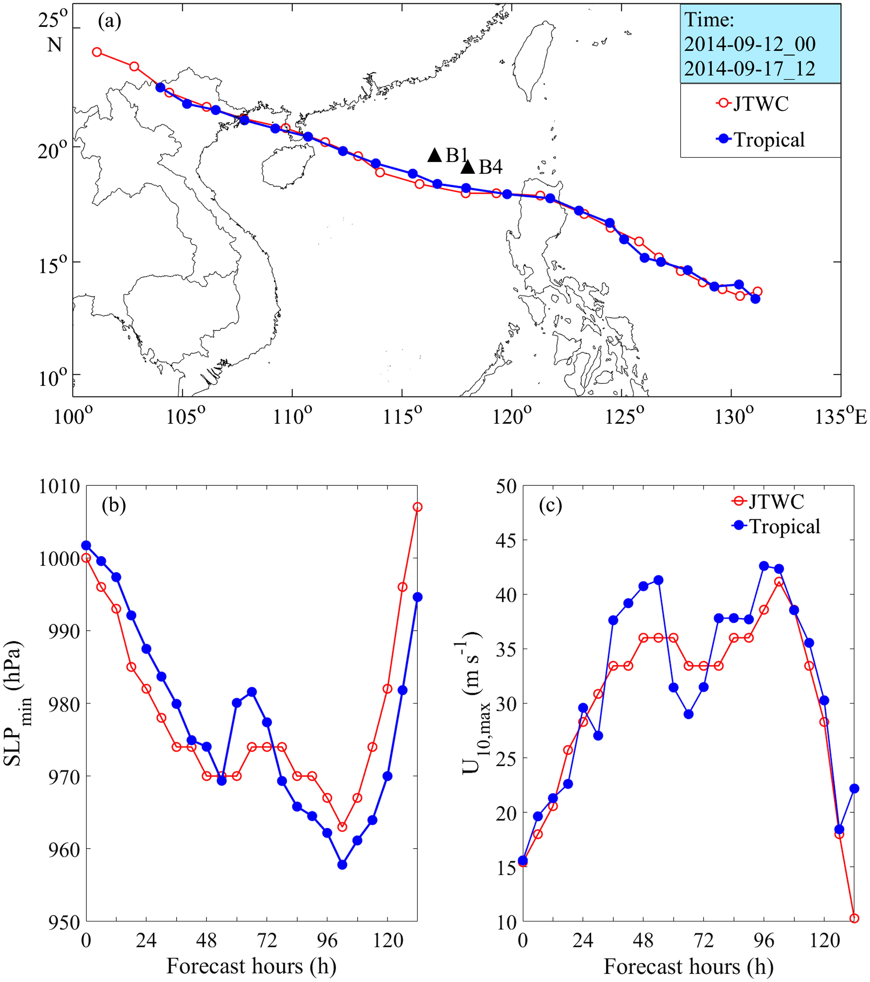
Fig. 3.
(a) Observed best track of Kalmaegi from JTWC (red line) and the simulated track using ‘Tropical’ suite (blue line). (b) The minimum sea surface pressure, with lines as defined in (a). (c) As in (b) but for the maximum 10 m wind speed.
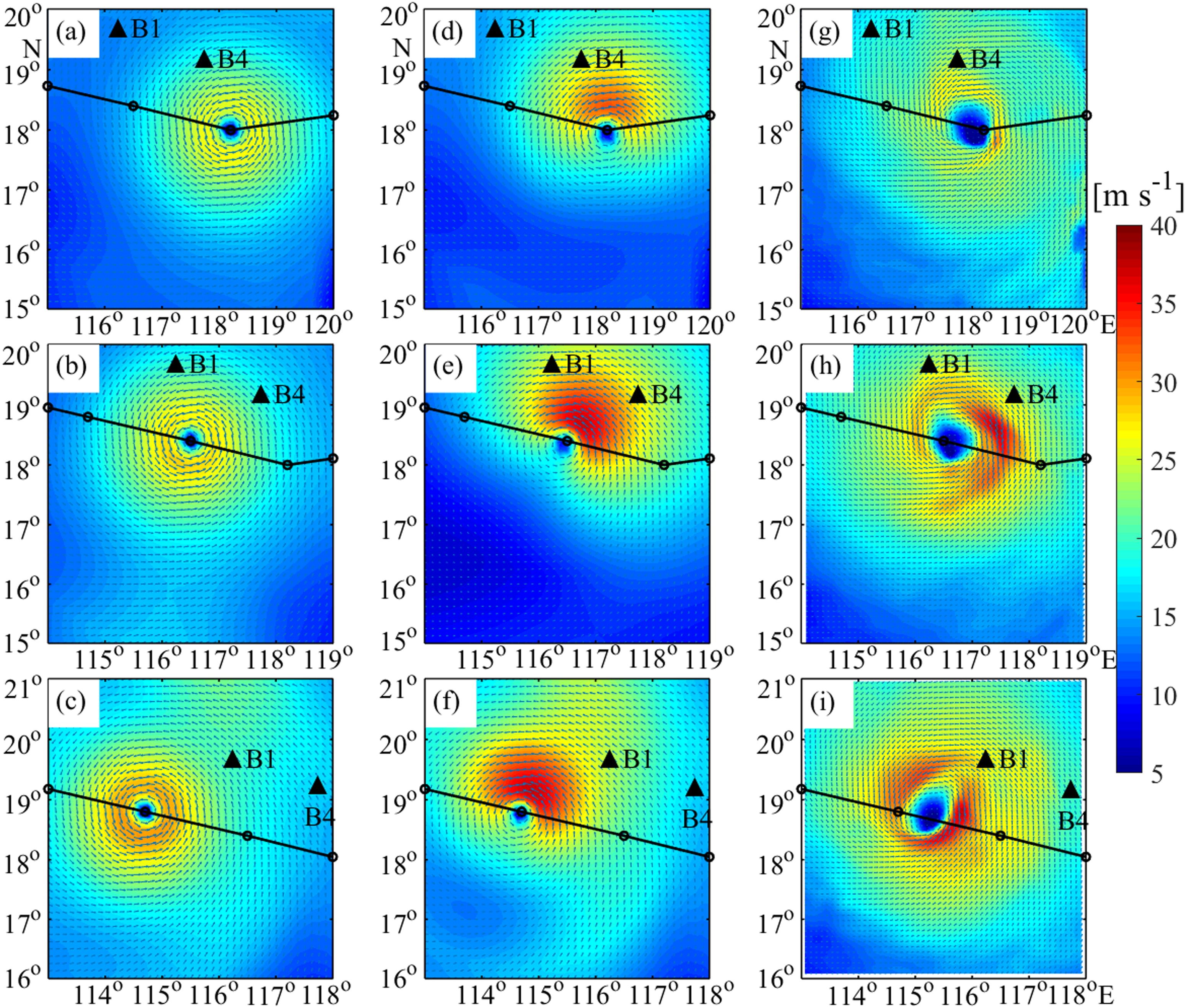
Fig. 4.
Comparison of spatial distributions among symmetric wind field (left column: a–c), asymmetric wind field (middle column: d–f), and WRF output (right column: g–i) at 0000 UTC 15 Sep (top row: a, d, g), 0600 UTC 15 Sep (middle row: b, e, h) and 1200 UTC 15 Sep (bottom row: c, f, i). Buoys location are marked by black triangular and the center of the typhoon are marked by black circle.
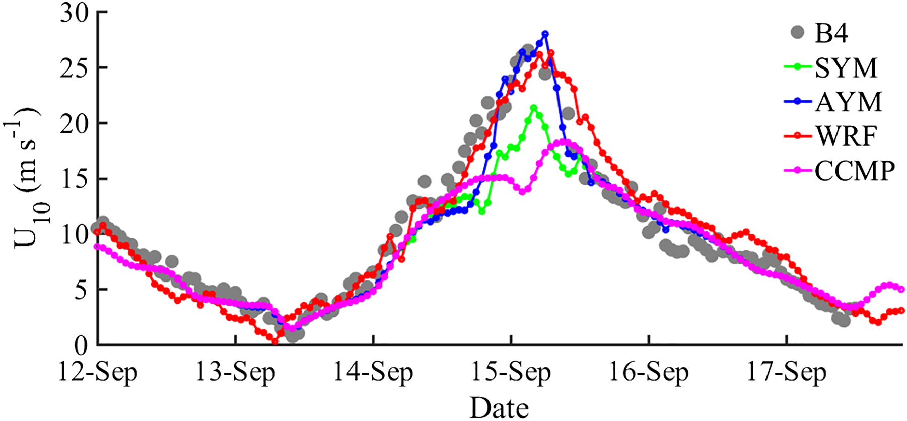
Fig. 5.
Time series of 10 m wind speed from CCMP and three wind fields versus observed data at B4.
Table 2.
Experimental design.
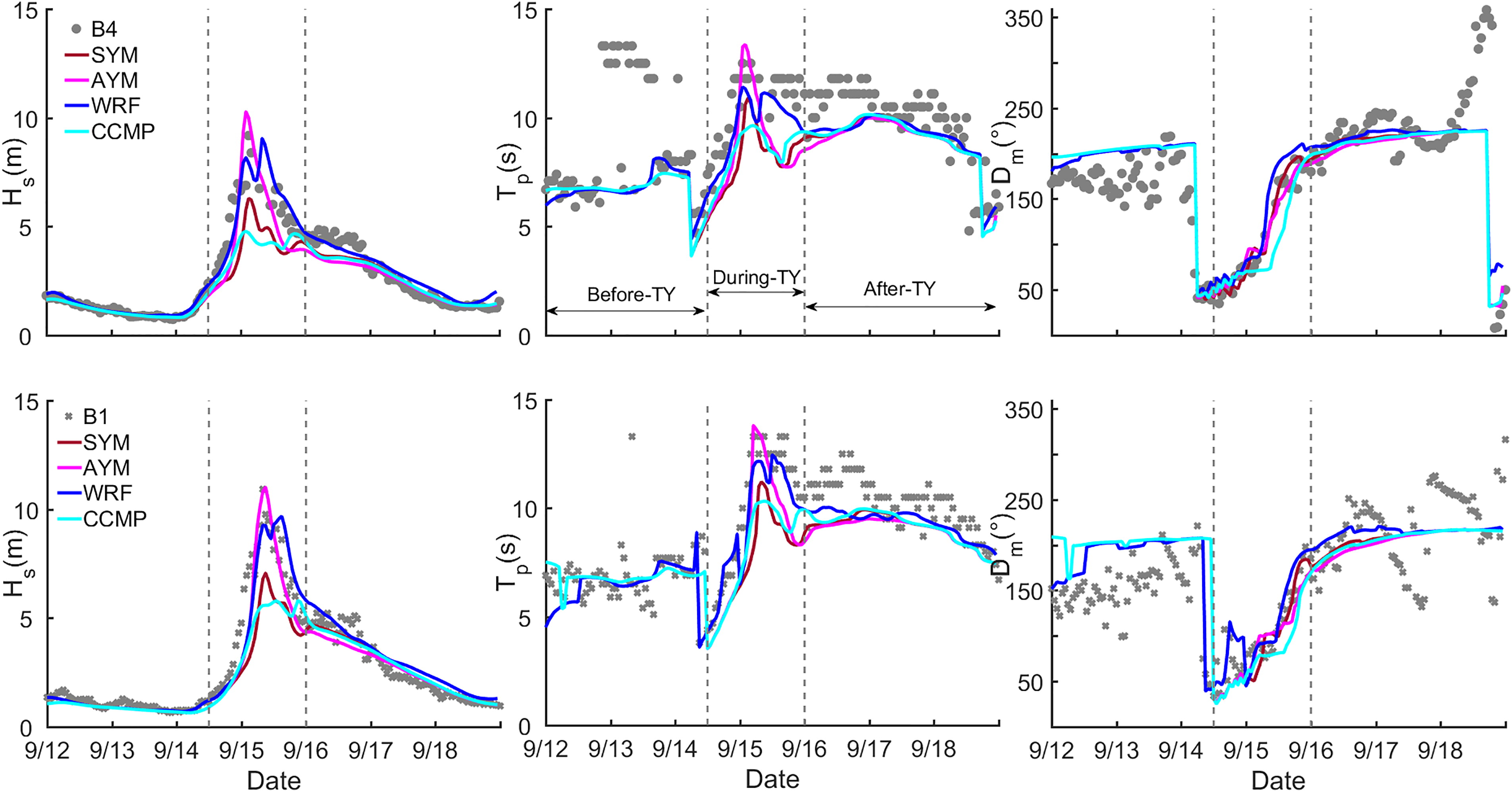
Fig. 6.
Time series of simulated (m) (left column), (s) (middle column), and (°) (right column) vs. the observed data at: B4 (top row) and B1 (bottom row).
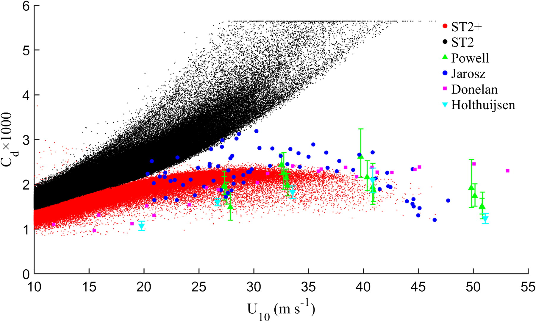
Fig. 7.
Wind stress coefficient obtained from ST2+ case (red dots), ST2 case (black dots) and field observations (e.g. Powell (with error bars); Jarosz; Donelan; Holthuijsen (with error bars)) vary with 10 m wind speed.
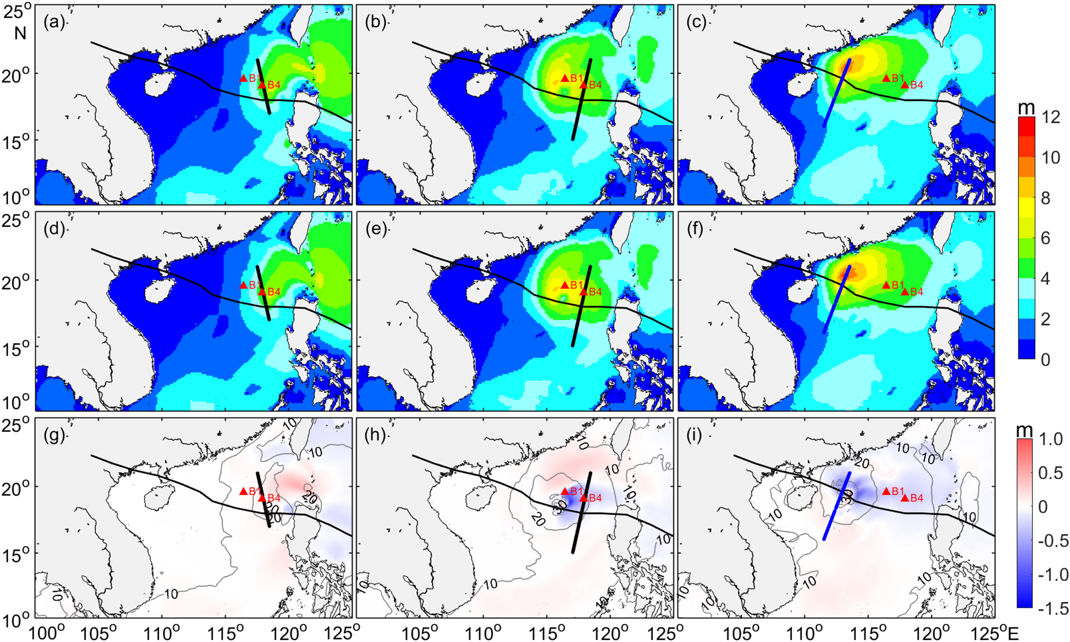
Fig. 8.
Spatial distribution of driven by WRF’s output among ST2+ case (top row: a–c), ST2 case (middle row: d–f) and differences between two cases (bottom row: g–i) at 2200 UTC 14 Sep (left column a, d, g), 1000 UTC 15 Sep (middle column b, e, h) and 2100 UTC 15 Sep (right column c, f, i). The heavy solid lines denote the track of typhoon. 10 m wind speed contours are showed with grey lines in g, h, i (contour intervals of the wind field are 10 m s−1). Bold dashed lines from left column to right column denote scanning paths from Saral-707 (black), Saral-722 (black), and Jason-2 (blue) at corresponding moment, respectively.
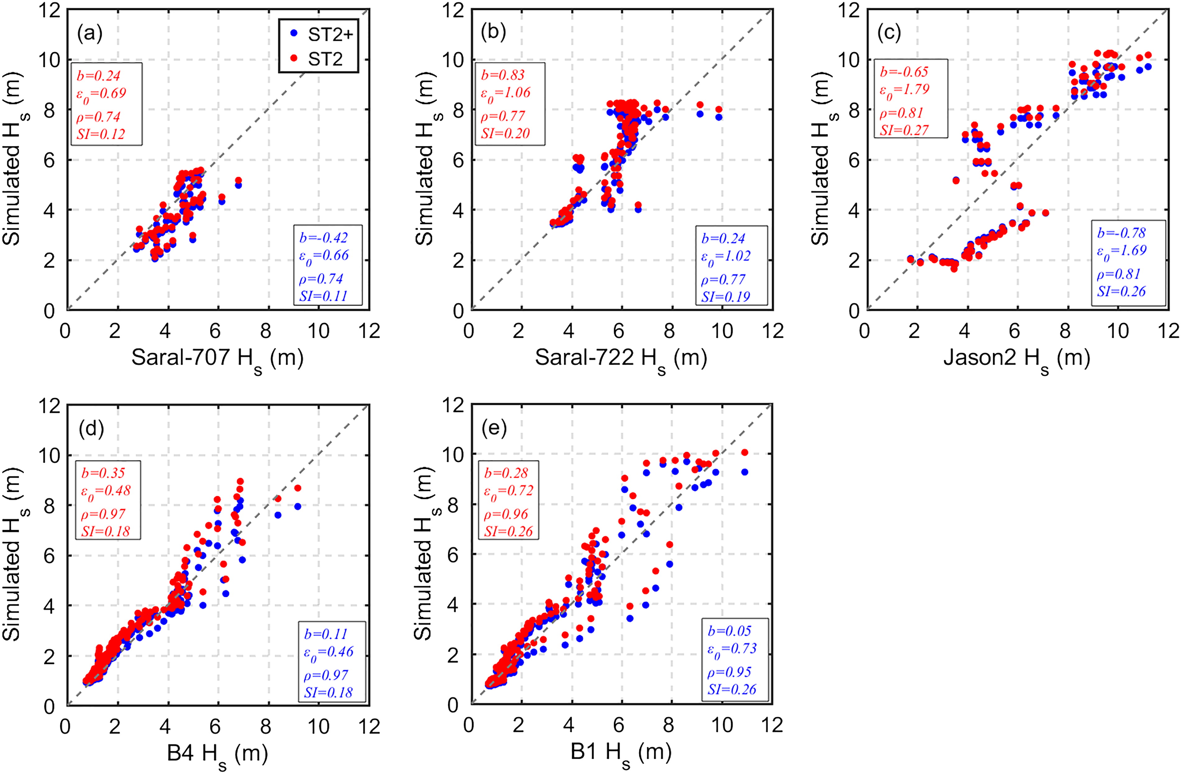
Fig. 9.
Comparison between the calibration results for the measurements according to Eqs. (1–2) and the simulated results from ST2+ (blue dots) and ST2 (red dots), respectively. (a–c) Saral-707, Saral-722 and Jason2, respectively. Similarity, comparison between buoy-based measurements and the simulated results are showed in (d) and (e). Error statistics for bias ,RMSE , correlation coefficient , and scatter index are given inset. The dashed line is 1:1 line.
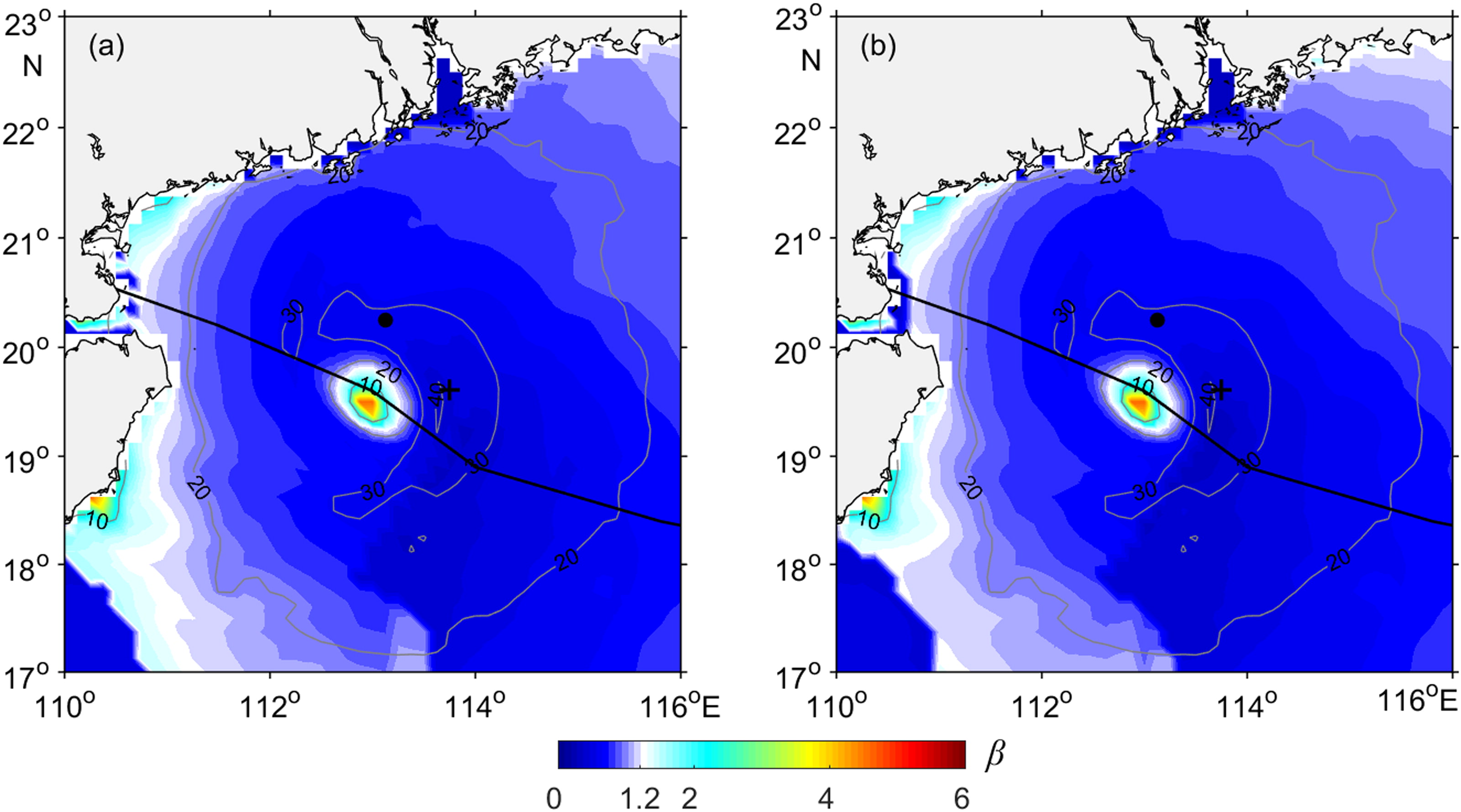
Fig. 10.
Spatial distribution of wave age (coloured) between ST2+ (a) and ST2 (b) cases at 2100 UTC 15 Sep, respectively. The heavy solid lines denote the track of typhoon. Wind speed contours are showed with grey lines, black ‘+’ and black ‘●’ denote the position of and at this moment, respectively.