
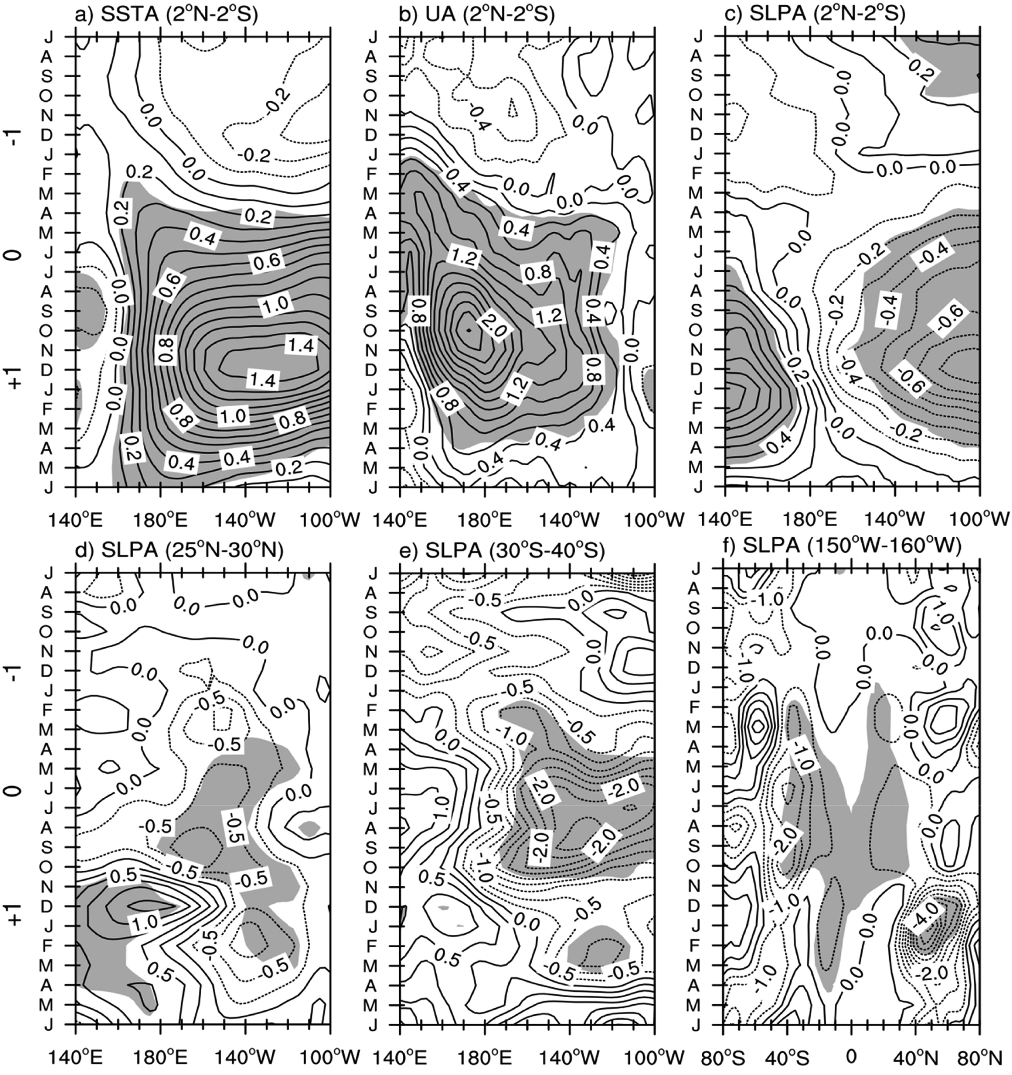
Fig. 1.
The El Niño composite for SSTa (a, unit: K), surface zonal wind anomalies (b, unit: ms−1), SLPa (c, unit: hPa) averaged between 2°N and 2°S; SLPa averaged between 25°N and 30°N (d), averaged between 30°S and 40°S (e), averaged between 150°W and 160°W (f) from July of −1 year to June of +1 year. The 0 years for the composite included 1965, 1972, 1976, 1982, 1986, 1987, 1991, 1994, 1997, 2002, 2003, 2006, 2009, 2014, 2015. Shaded areas indicate significance at 95%.
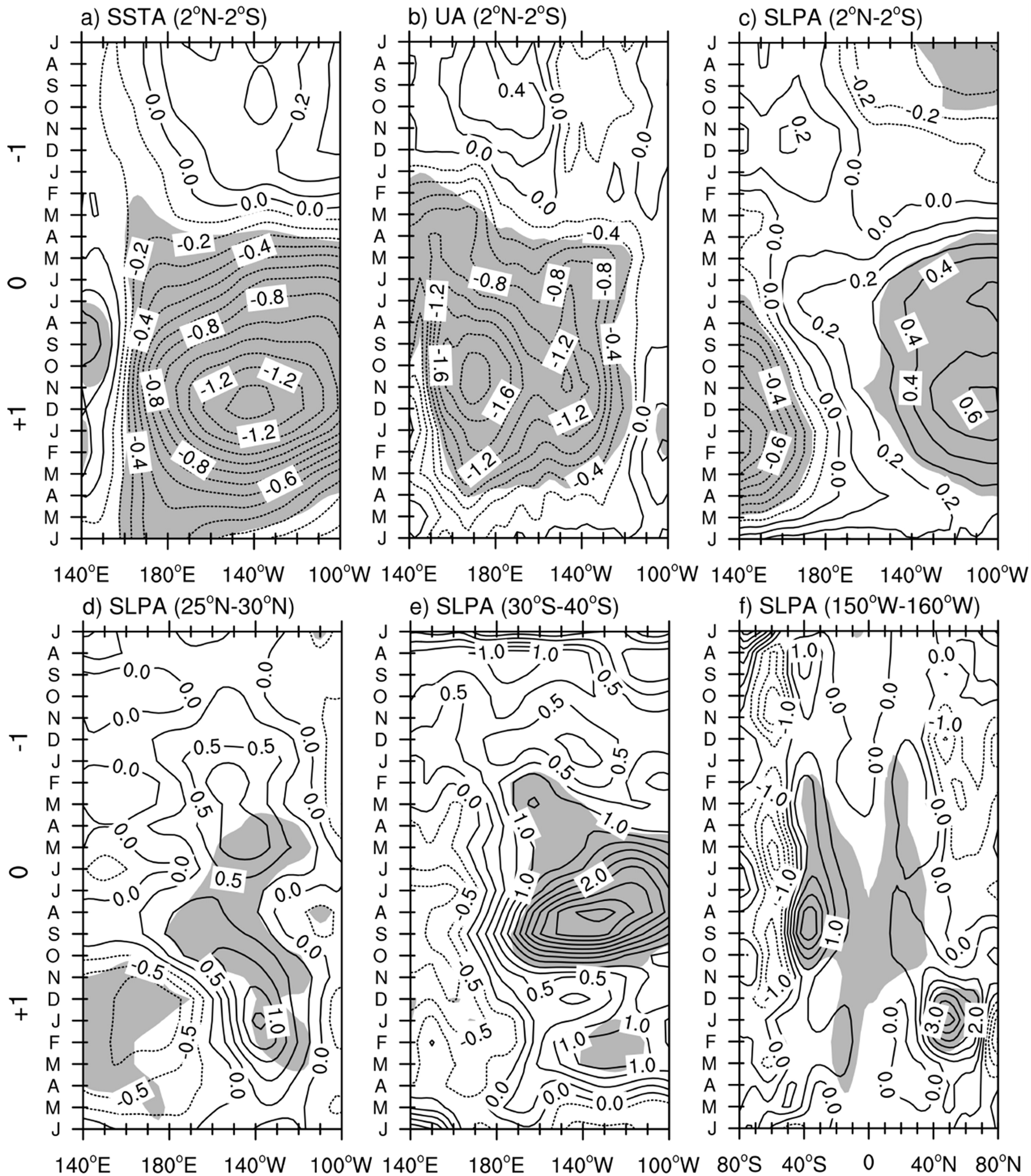
Fig. 2.
Same as Fig. 1, except for the La Niña composite for the years of 1964, 1967, 1970, 1971, 1973, 1974, 1975, 1984, 1988, 1995, 1996, 1998, 1999, 2007, 2010.
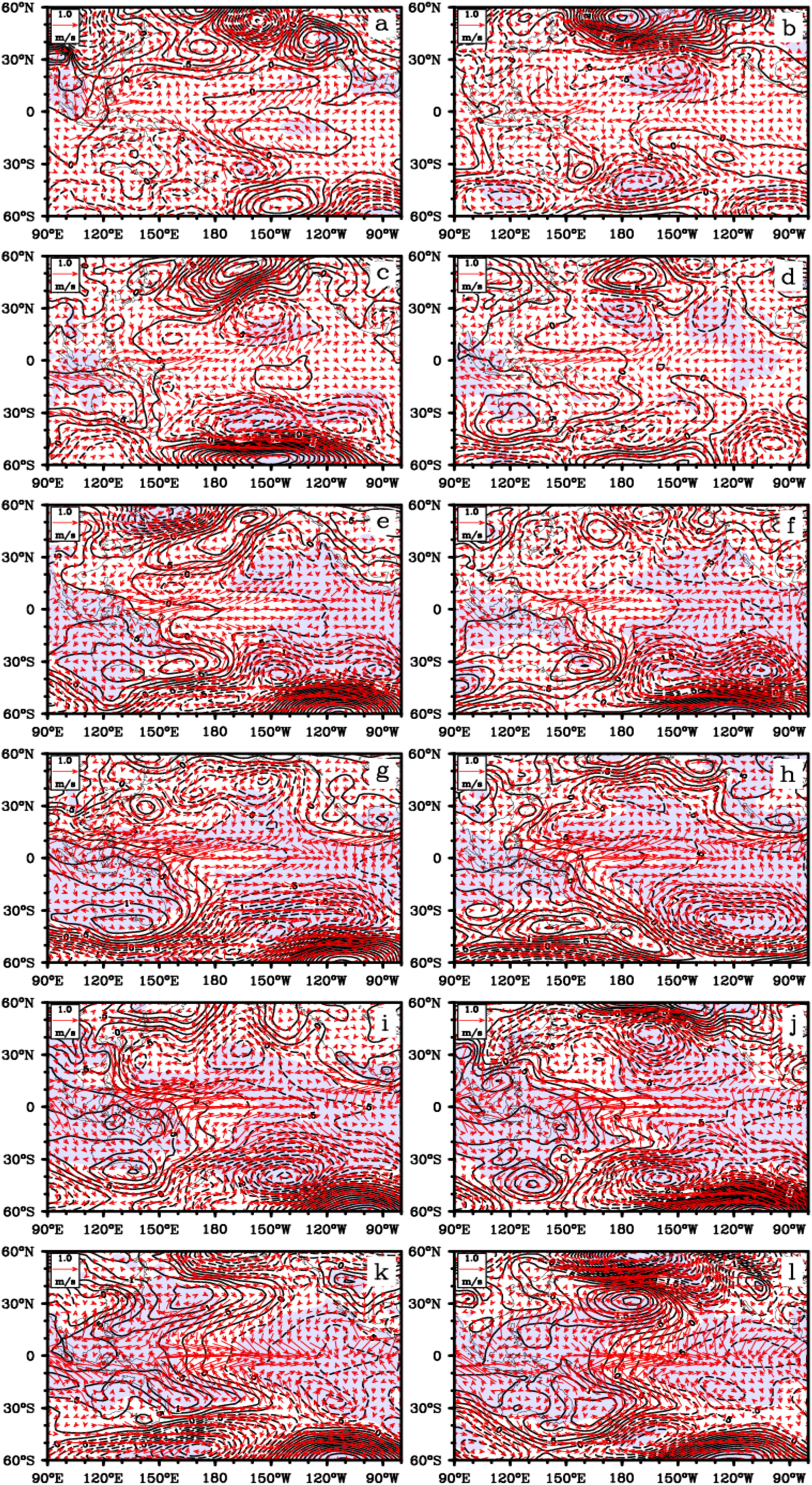
Fig. 3.
Distributions of SLPa (unit: hPa) and surface wind vector (unit: ms−1) anomalies for El Niño composite from January to December (a–l). Shaded areas indicate the significance at 95%.
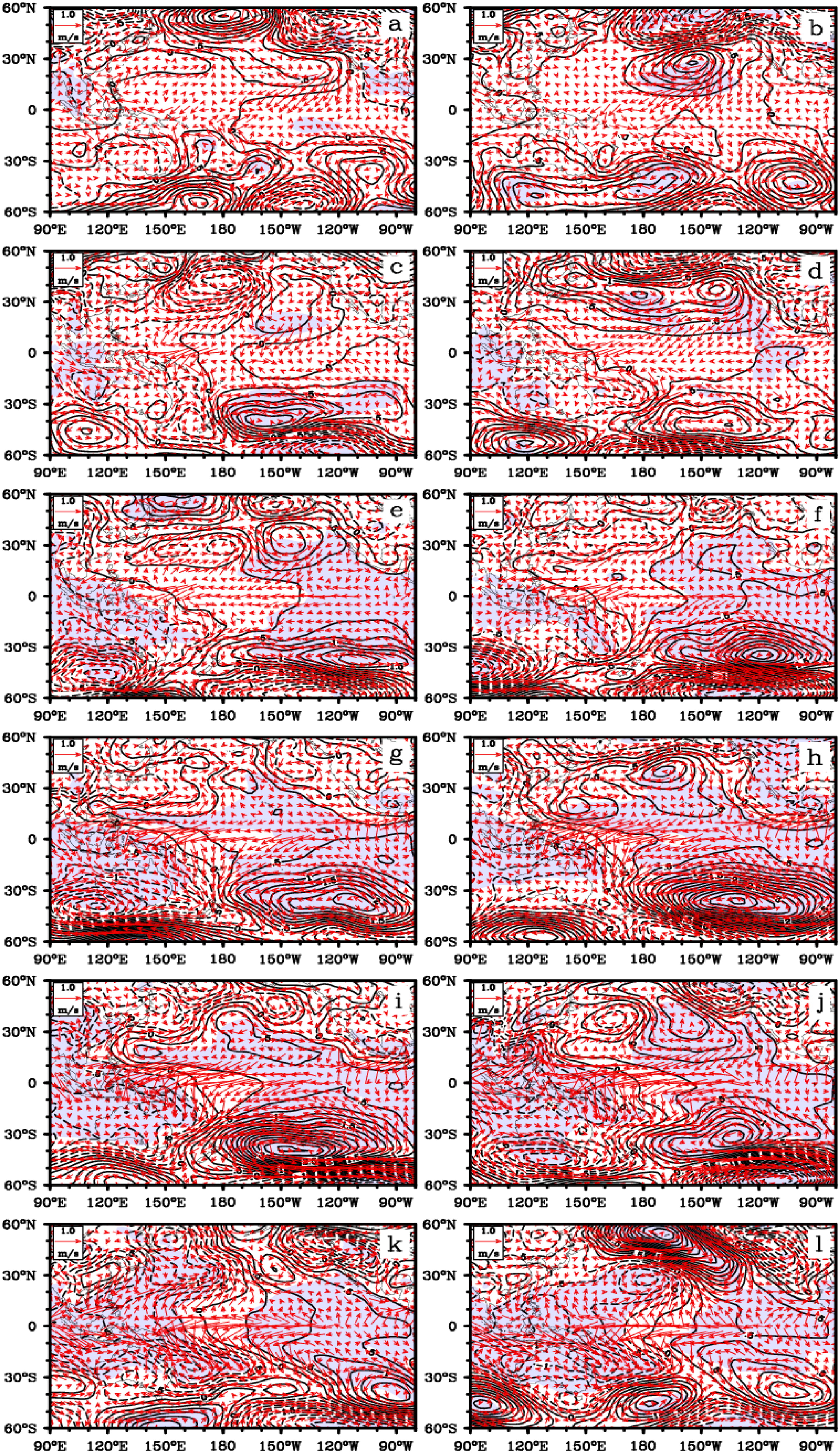
Fig. 4.
Same as Fig. 3, except for the La Niña composite.
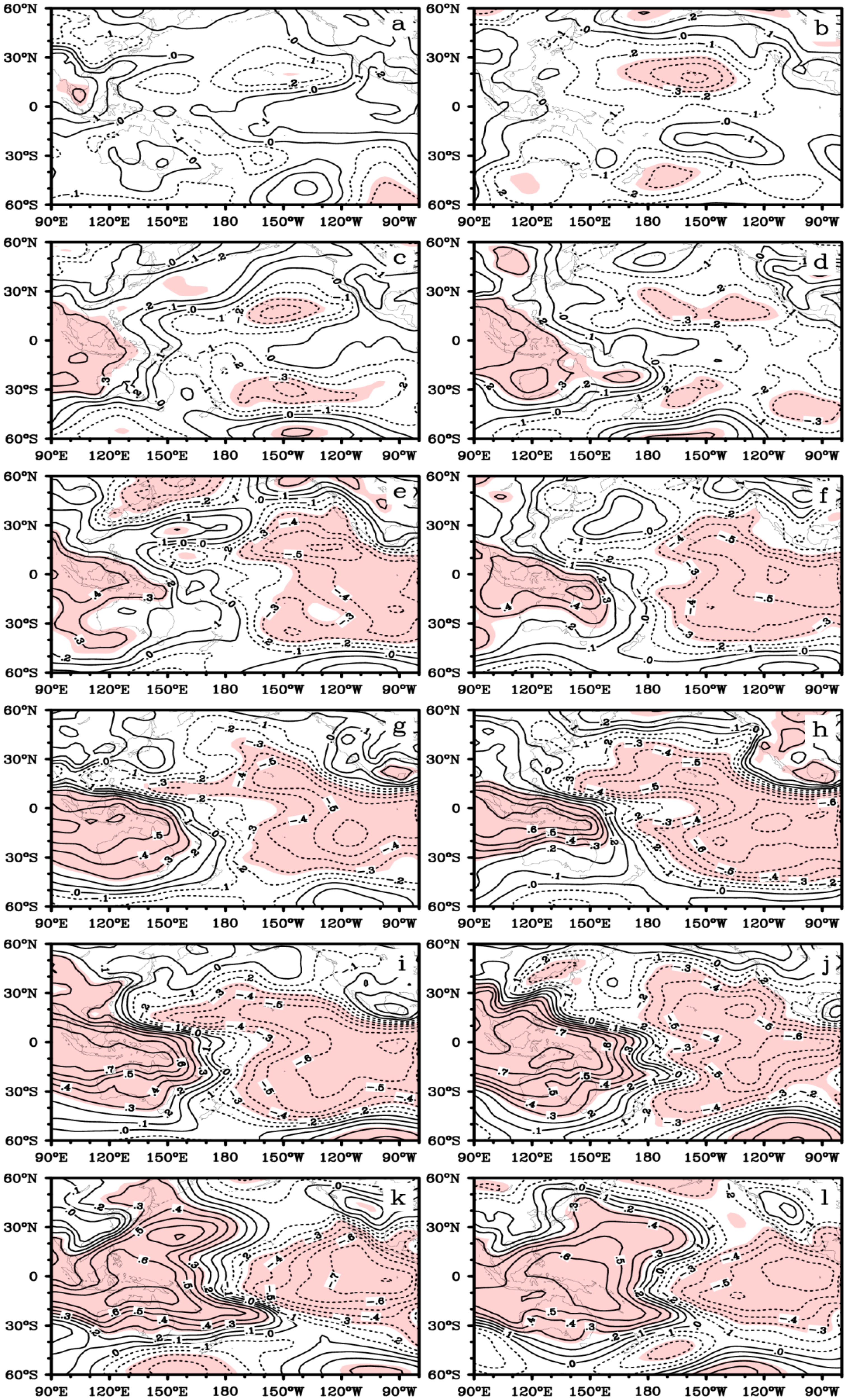
Fig. 5.
The correlation between SLP and SST3DJF from January to December. Shaded areas indicate the significance at 95%.
Table 1.
Correlation coefficients between I-N and SST3DJF.
[i] The cor.2, cor.3… show coordinates for the accumulative months of I-N. For example, cor. 2 vs. cor. 5 means the correlation between I-N2-5 and SST3DJF and cor.3 vs. cor.10 means the correlation between I-N3-10 and SST3DJF, and so on. Italic values signify significance above 99% confidence level.
Table 2.
Same as in Table 1 except for the correlations involving I-S.
Table 3.
Same as in Table 1 except for the correlations involving I-All.
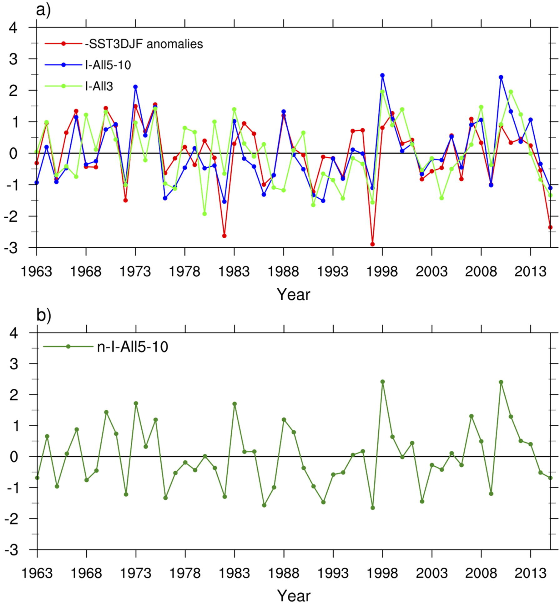
Fig. 6.
The evolution of I-All3, I-All5-10, and SST3DJF multiplied by −1 (a) and n-I-All5-10 (b) from 1963 to 2015. The data were normalised by their own standard deviations.
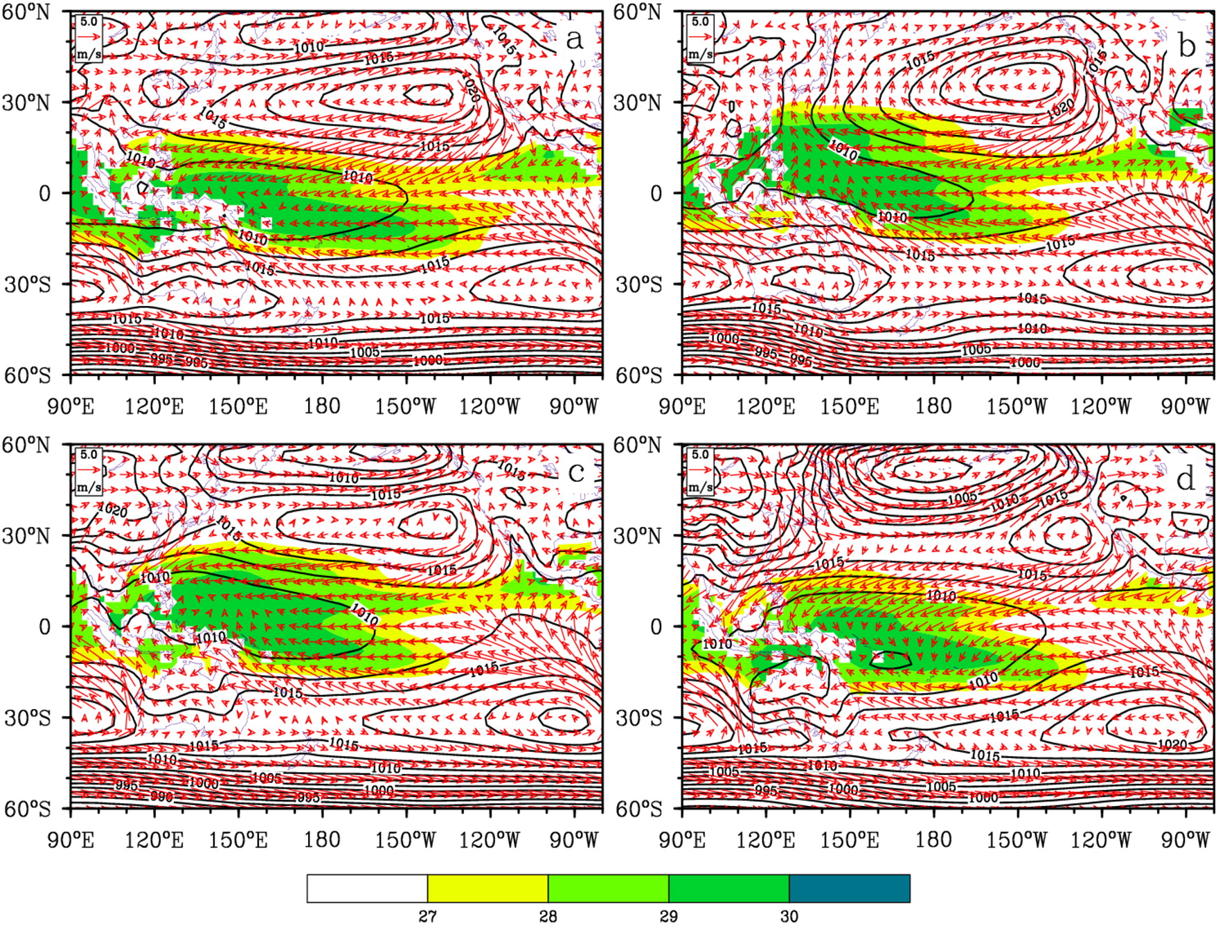
Fig. 7.
Climatic distribution of monthly SLP, surface wind vector and SST over 27 °C averaged from 1963 to 2015 for MAM (a), JJA (b), SON (c) and DJF (d).
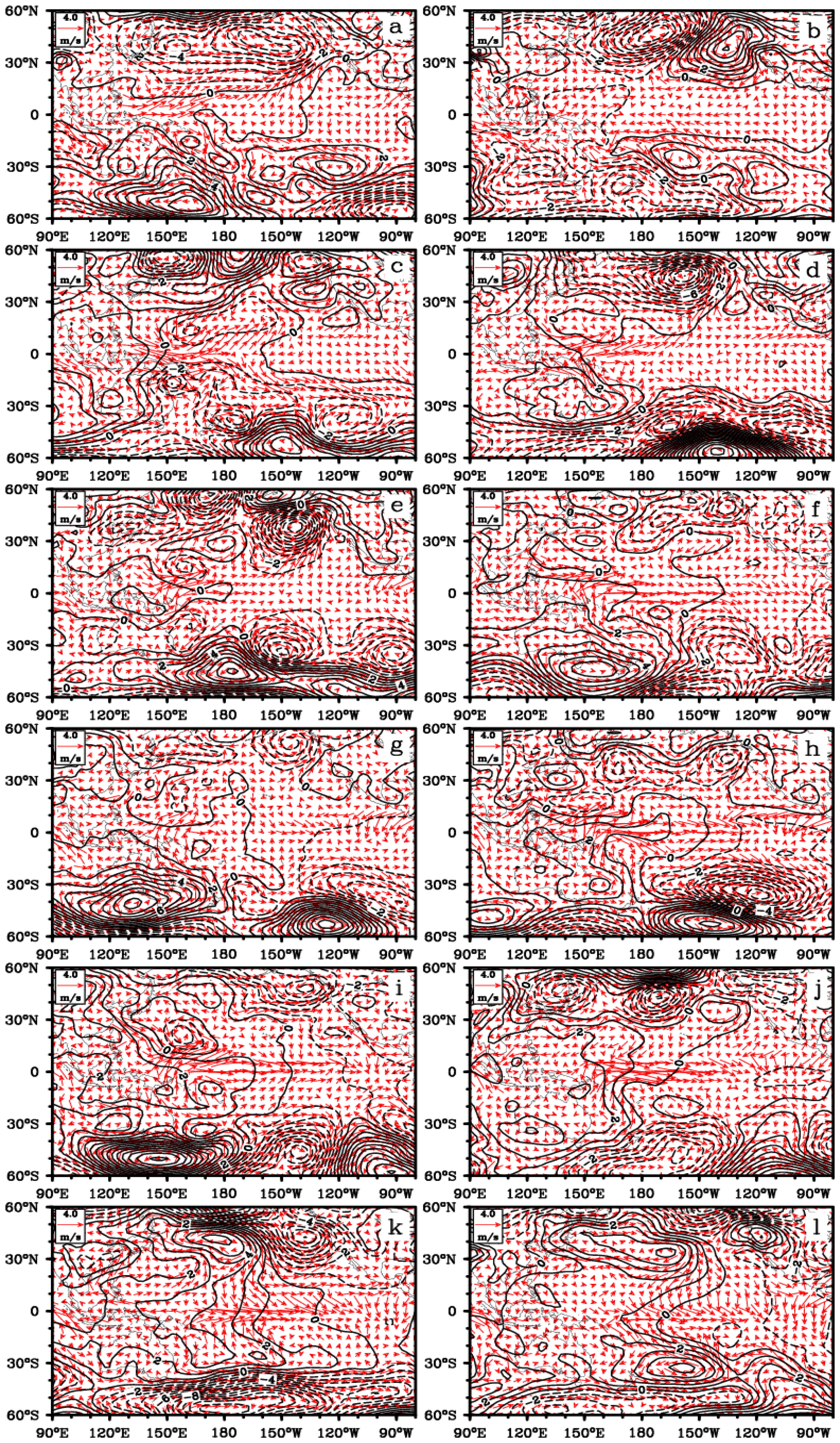
Fig. 8.
Same as Fig. 3, except for the period in 1997.
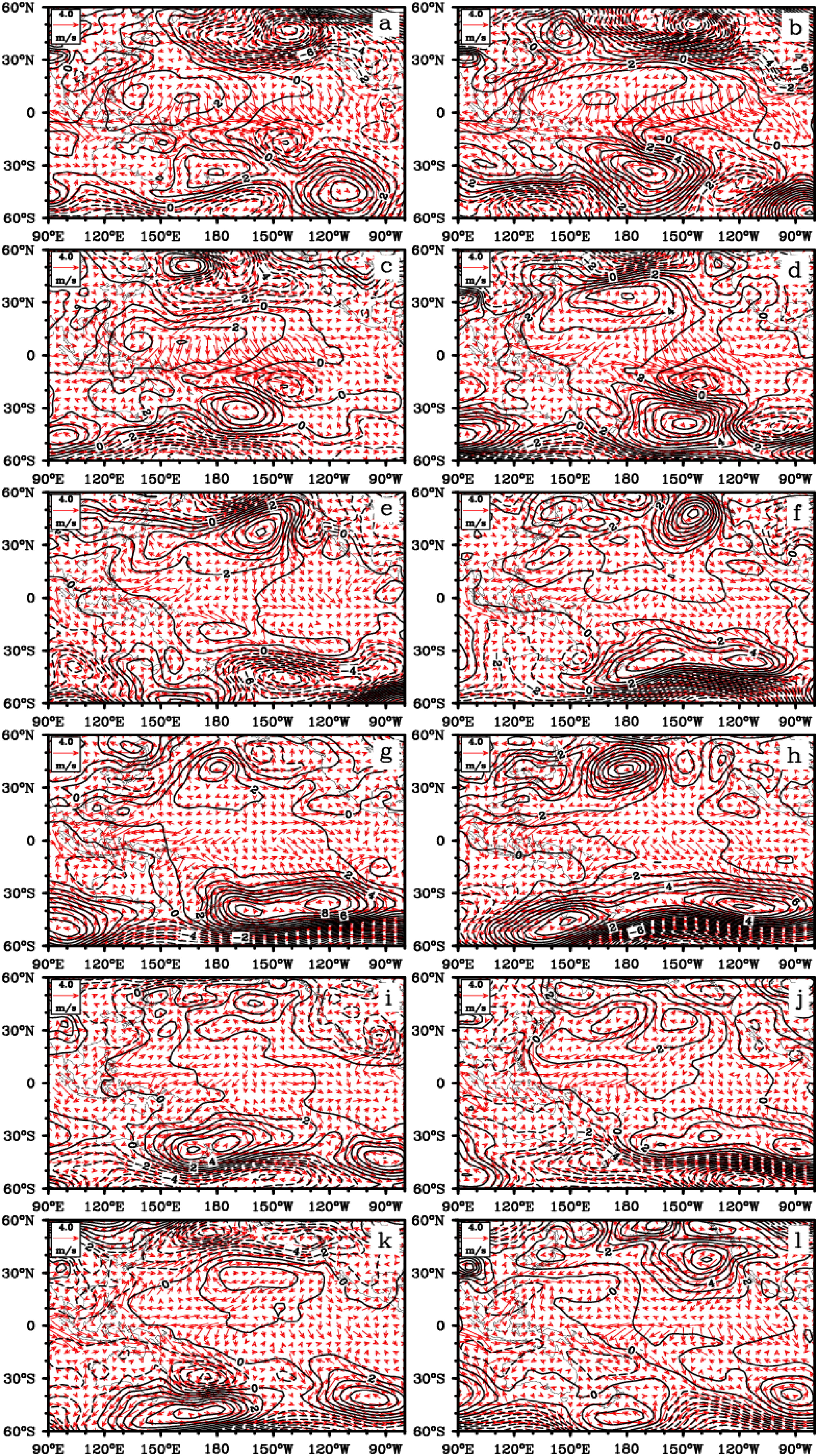
Fig. 9.
Same as Fig. 8, except for the period in 1998.
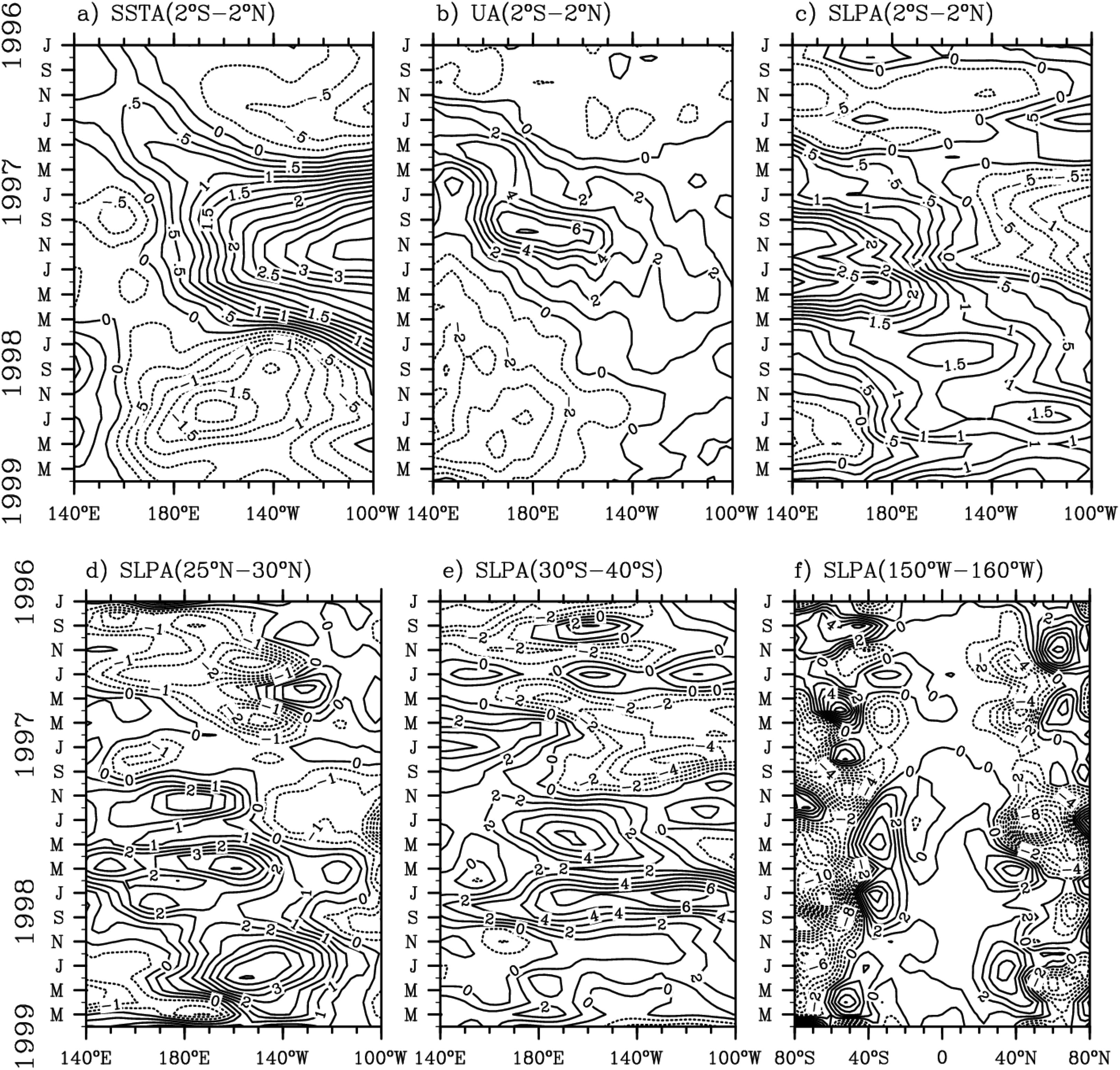
Fig. 10.
Same as Fig. 1, except for the period from July 1996 to June 1999.