
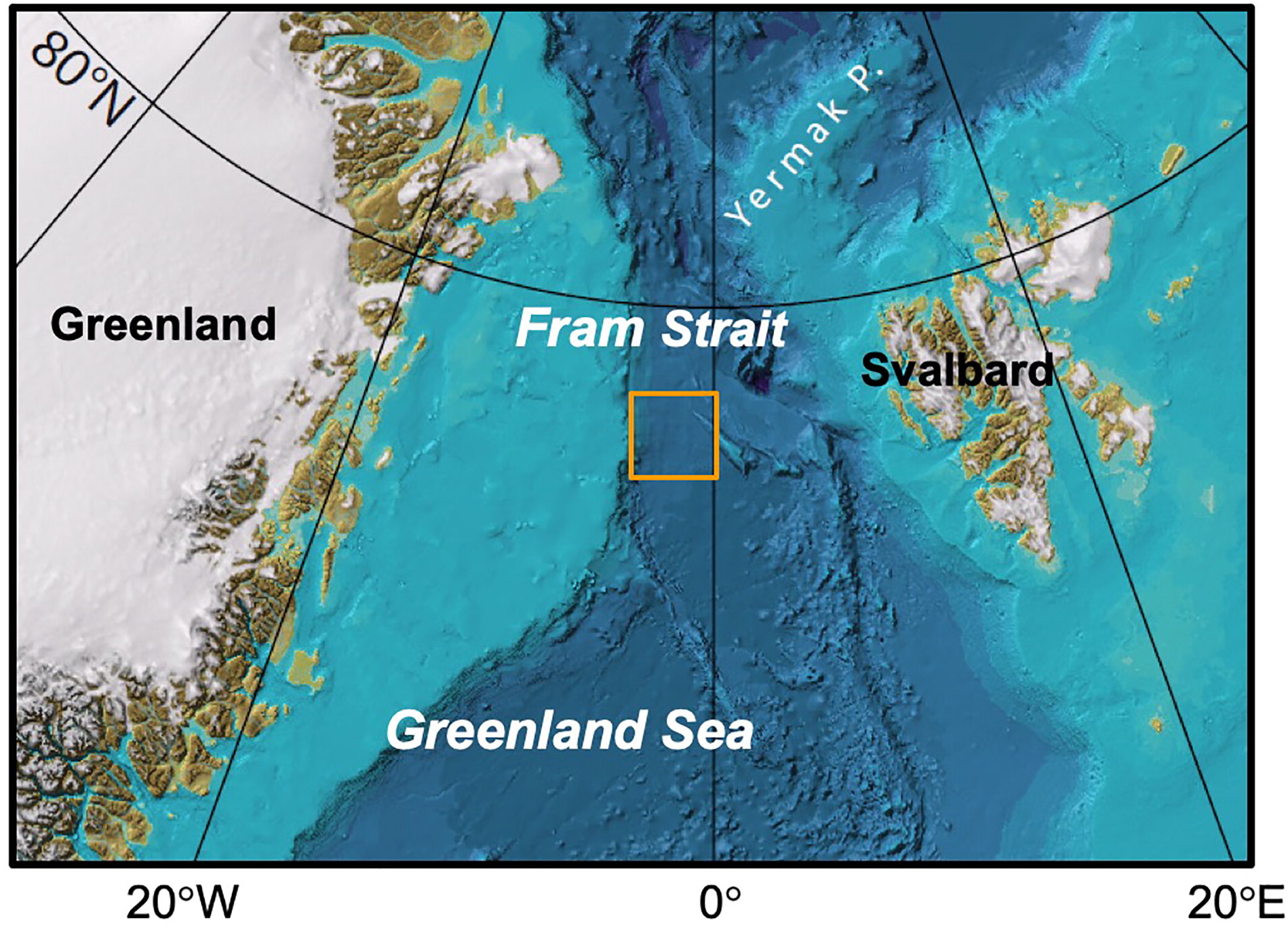
Fig. 1.
Bathymetric map of the Fram Strait area and northern Greenland Sea. Yellow frame indicates the experiment area as detailed in Fig. 2a. Base map is from the International Bathymetric Chart of the Arctic Ocean (IBCAO) (Jakobsson et al. 2012).
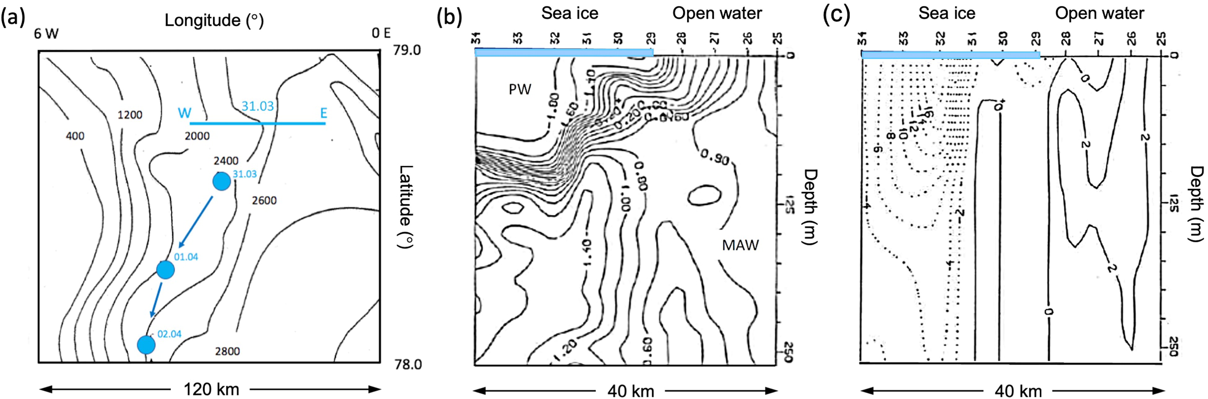
Fig. 2.
a, Location and bathymetry (in metres) of the experimental area, drift of the array during 31 March – 2 April (blue dots), and oceanographic section on 31 March (blue line marked W–E). b, Temperature section across the East Greenland Sea Polar Ocean Front, PW is cold Polar Water of less than –1.8 °C; here, only the isotherms between –1.0 °C and +1.4 °C are shown for each 0.1 degree C. MAW is warm Modified Atlantic Water. c, Calculated geostrophic current in cm/s across the section with 0 reference level at 1000 m the dotted lines correspond to the southward current; full lines correspond to the northward current in cm/s contoured for each 2 cm/s from –20 cm/s to –2 cm/s southwards to 2 cm/s northwards. Sea-ice cover is shown by the thick blue line at the surface. The section is 40-km long with station spacing of 4.4 km.
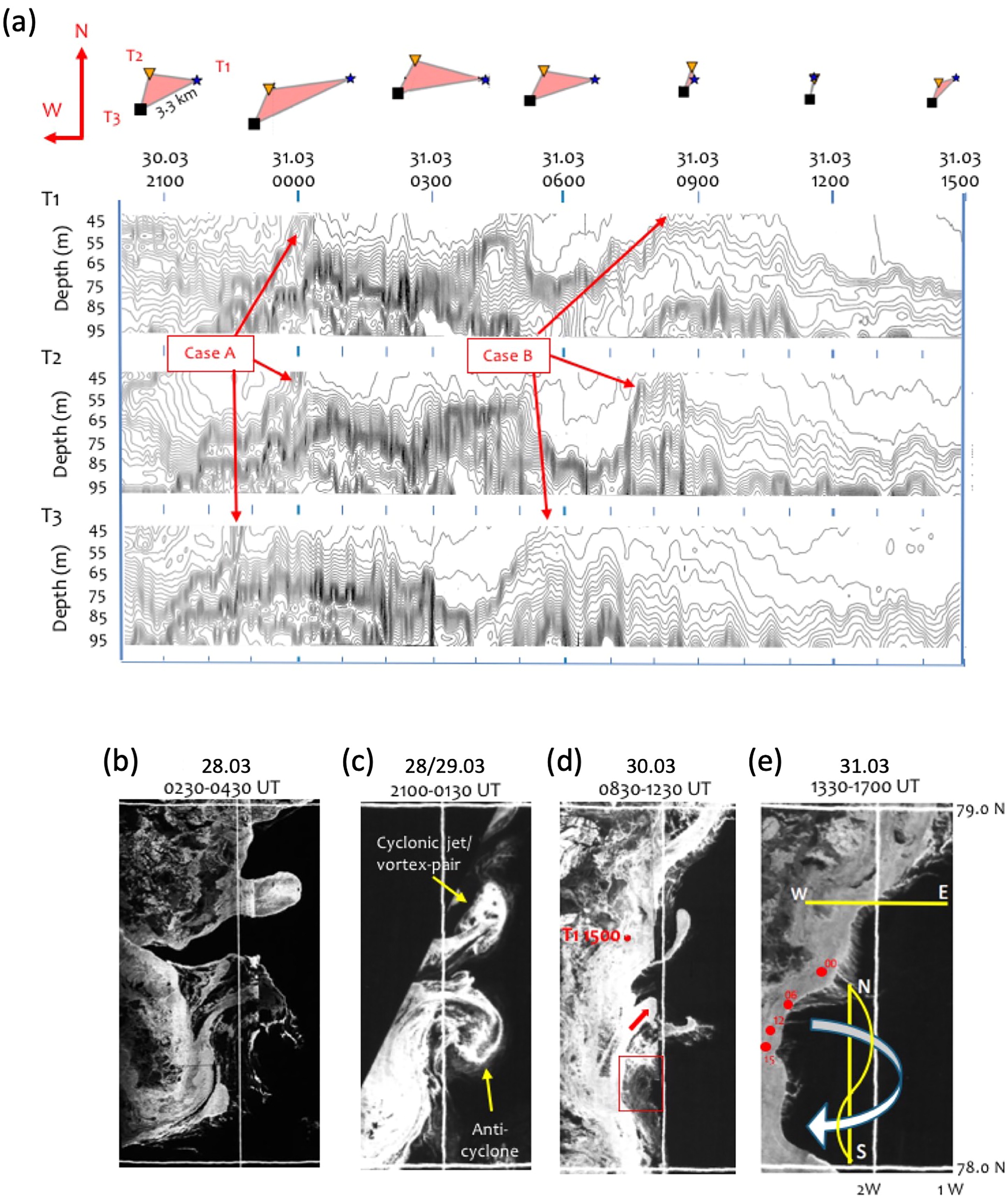
Fig. 3.
Observations of internal waves and ice-ocean eddies. a, Isotherms between –1.8 °C and 1.8 °C (shown with an interval of 0.1 °C) in the thermocline layer between 45 and 95 m obtained every 2 minutes by the triangle (plotted above with 3-hour interval) with thermistor chains, spaced each 5 m. The arrival times for the two local wave crests detected during 30–31 March are marked as Case A and Case B. b–e, Synthetic Aperture Radar (SAR) images from 28–31 March. Red dot marks the deployment of the array on 30 March, and red arrow indicates the flow of the ice in the anticyclonic eddy; the red box shows the area where the internal waves are observed (see Fig. 3a). Red dots in E show the array on 31 March at 00:00, 06:00, 12:00 and 15:00. Yellow lines are the East (E)–West (W) oceanographic section obtained on 31 March (in Fig. 2b,c) and the North (N)–South (S) section obtained on 2 April. Schematically, the E–W geostrophic profile is shown by a curved yellow line and the circular white arrow shows the anticyclonic eddy. See Fig. 4.
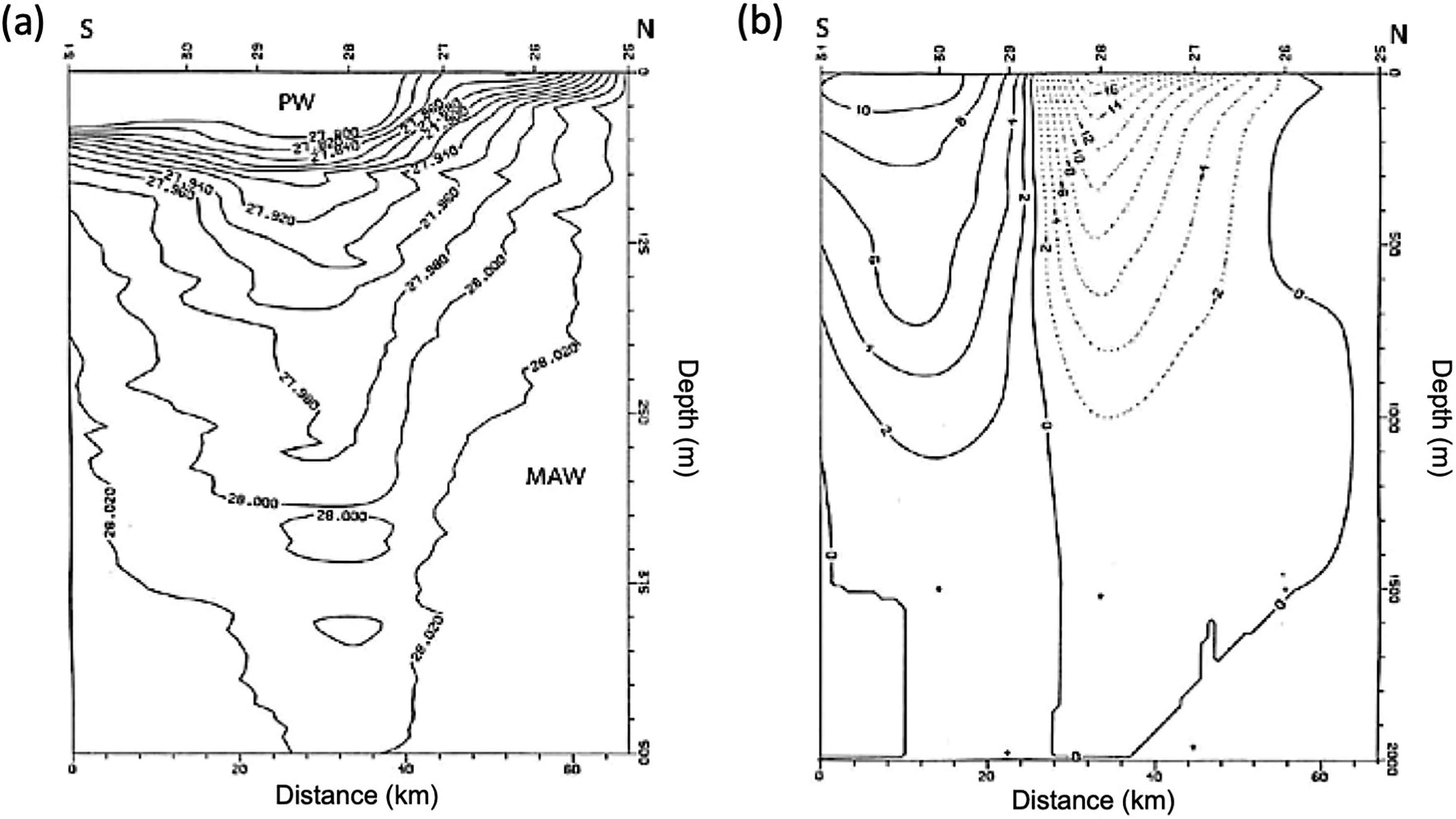
Fig. 4.
The anticyclonic eddy characteristics. a, Density section of the North (N)–South (S) section on 2 April shown in Fig. 3e. b, Geostrophic current in the N–S section with 0 reference level at 2000 m. Dotted lines: eastward current; full lines: westward current in cm/s. Note the different y-axis scale for the depth, 500 m for a and 2000 m for b. The section is 65-km long and with station spacing of 8–11 km.
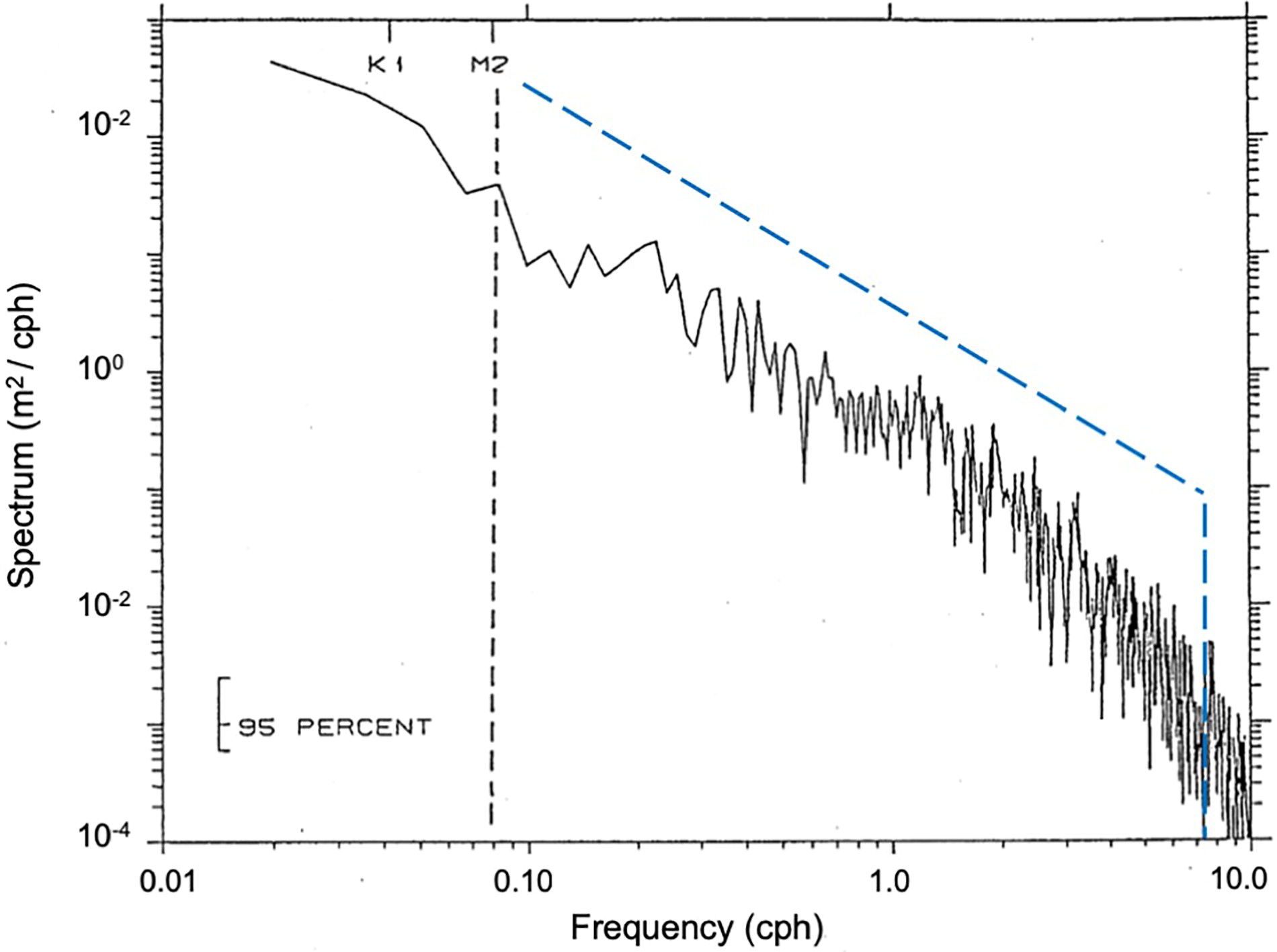
Fig. 5.
The vertical displacement spectrum computed from 30 March to 4 April of the temperature series from the thermistor T1 at 60 m, divided by the mean vertical temperature gradient of 0.10 degree C/m is compared to the Garrett-Munk spectrum, shown by the dotted line. The inertial period is close to the semidiurnal period for this latitude and the cut-off buoyancy frequency (N) is 6.5 cph. The spectrum is estimated by fast Fourier transformation (FFT), and the 95% confidence level is based on 10% tapering of the series and smoothing over five frequency bands with a resolution of 0.02 cph (Bloomfield,1976). The Garrett-Munk spectrum is plotted using a scaling factor R = 320 (exponent 2) cph and a cut-off frequency N= 6.5 cph (See Sandven and Johannessen (1987) for more details).
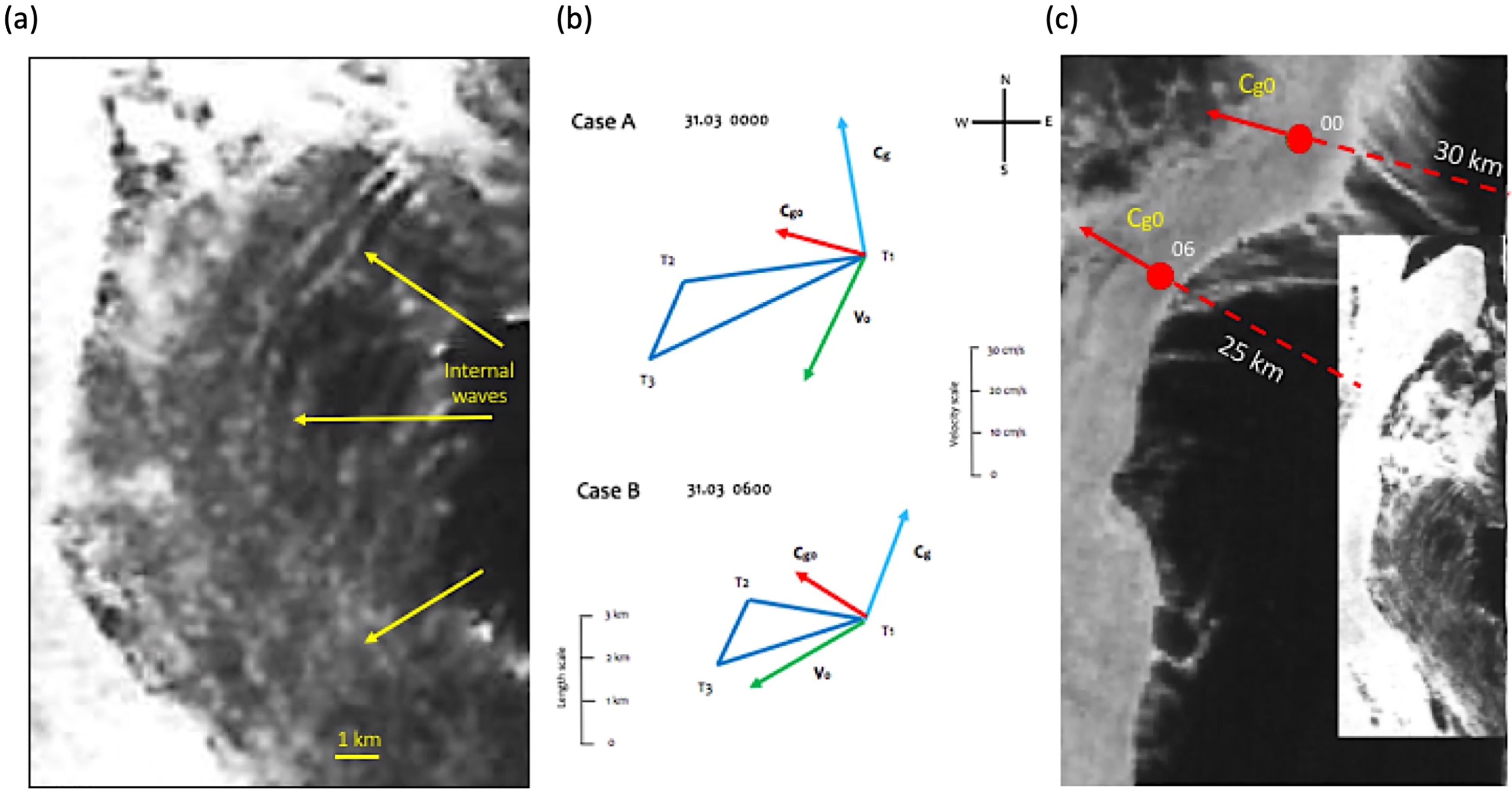
Fig. 6.
Imagery of internal waves and velocity calculations. a, Synthetic Aperture Radar (SAR) image of internal wave train with the wavelengths of 750–1000 m propagating at the western boundary of the anticyclone eddy (shown for 30 March by the slicks of curving bands of ice floes); for the location see red box in Fig. 3d. b, The triangle array T1-T2-T3 at 00:00 and 06:00 of 31 March, is the intrinsic group velocity of the internal wave train, is the average current velocity in the thermocline region, is the absolute group velocity relative to the ground. c, SAR image of 31 March. Red dots are the array positions at times 00 and 06 shown along with the absolute group velocity vectors, . Inserted is the part of the SAR image from 30 March, which includes the box shown in Fig. 3d. Dotted red lines from the array positions are backward extrapolation directions of the absolute group velocities hitting the internal waves on 30 March.