
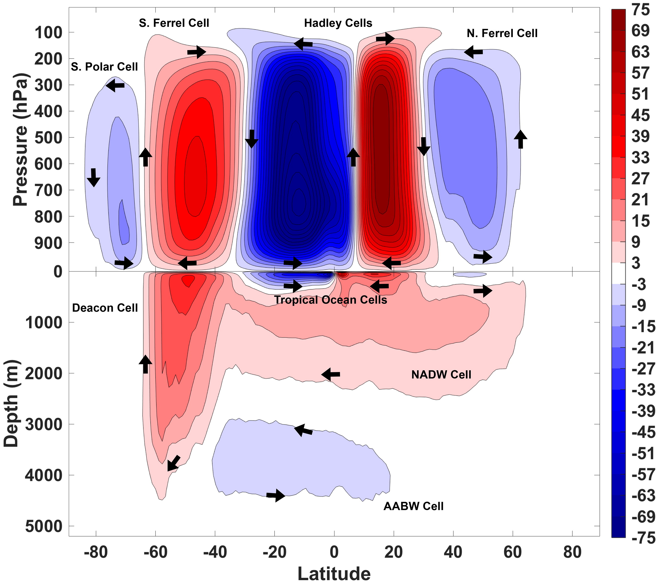
Fig. 1.
The global air-mass overturning stream function for the atmosphere (top panel) and global water-mass overturning stream function for the ocean (bottom panel). Arrows indicate the mass transport direction. N represents the Northern Hemisphere and S is used for the Southern Hemisphere. NADW stands for North Atlantic Deep Water and AABW represents Antarctic Bottom Water. All transports are in Sv ().
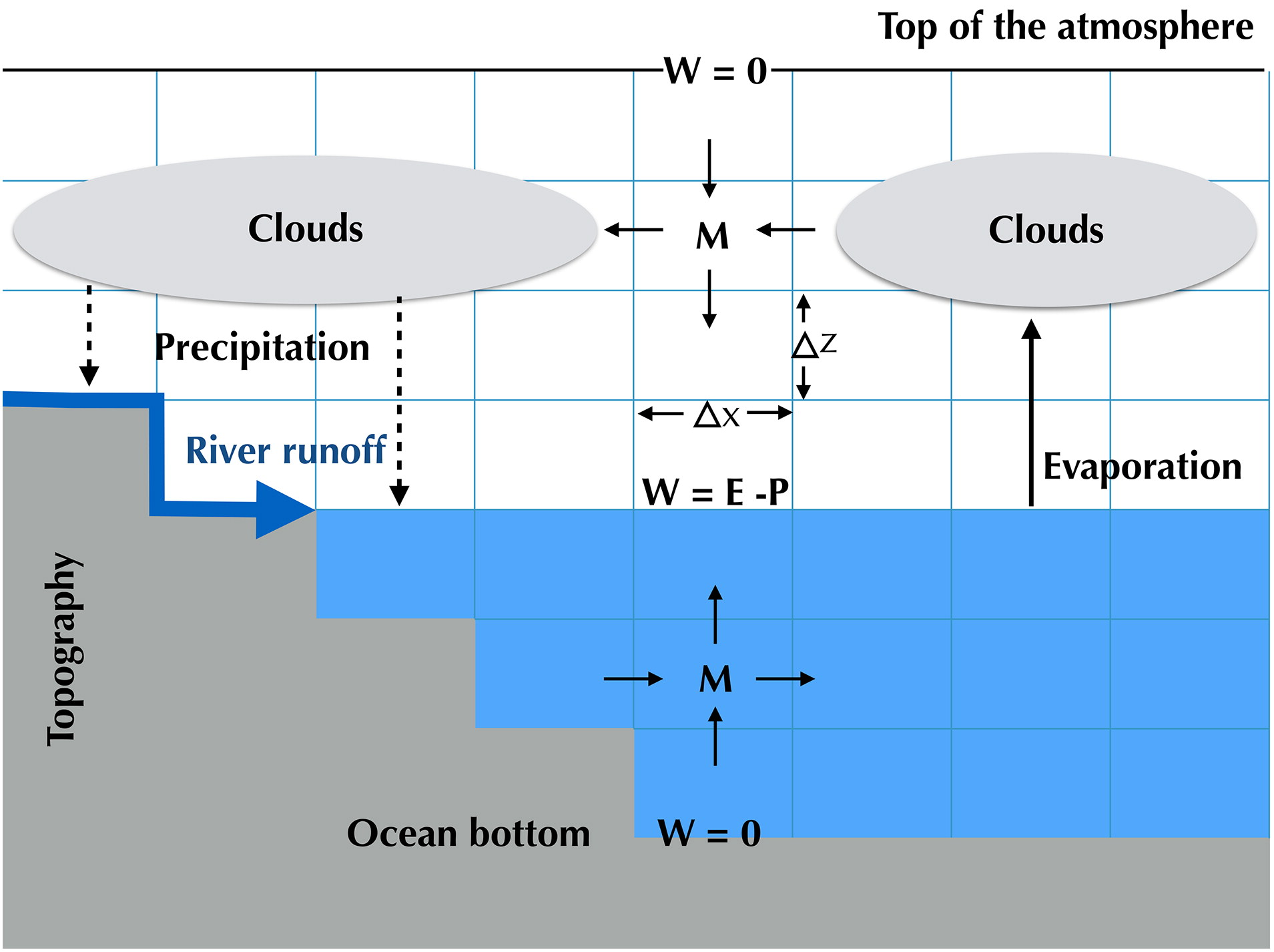
Fig. 2.
Sketch of the processes that mainly regulates the coupled ocean–atmosphere hydrological cycle. Also, this schematic diagram carries detailed information about the methodology that is described in methods. M is the atmospheric water-mass in a model grid box. W is vertical water-mass transport through the upper face of the grid box and at the surface this should equal the surface freshwater flux (). Conservation of water-mass yields that the rate of change of water-mass content of a box balances the water-mass fluxes though its faces.
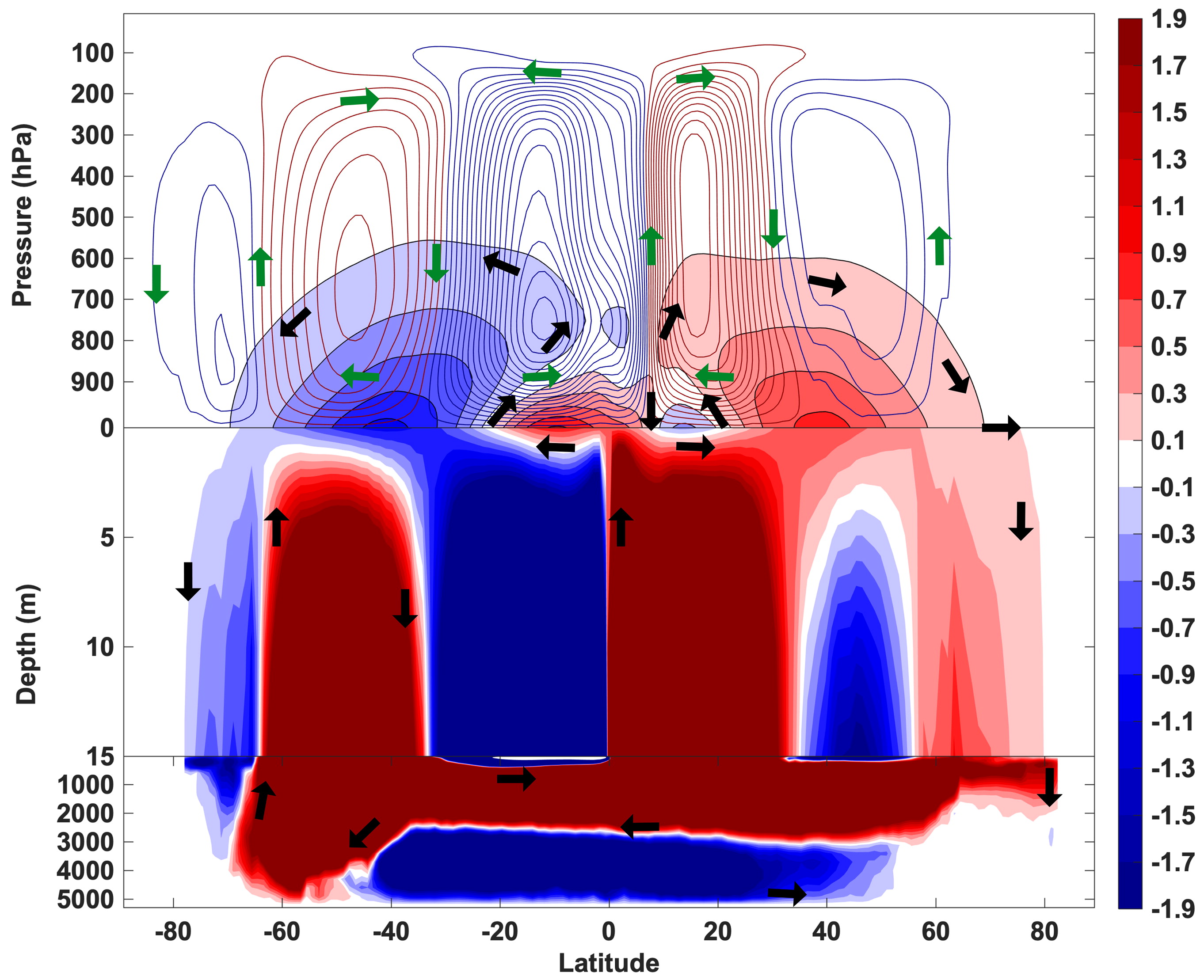
Fig. 3.
The global water-mass overturning stream function for the coupled ocean–atmosphere system superimposed with the global air-mass overturning stream function for the present day climate. Black arrows show the water-mass transport direction and green arrows indicate the air-mass transport direction. All transports are in Sv (). Note that the colour scale is saturated. Contour interval for air-mass transport is 6 Sv. The ocean water-mass overturning stream function here is the same as in Fig. 1 bottom panel, but with different contour interval and with a non-linear depth scale. There are two ocean model vertical levels in the stretched part of the graph from the surface to depth 15 m.
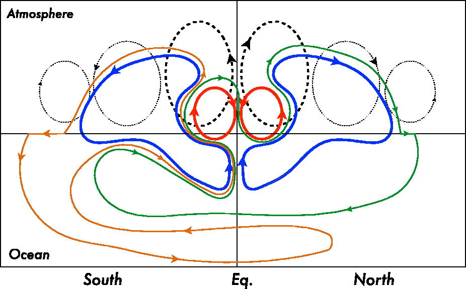
Fig. 4.
Schematic diagram of the ocean–atmosphere water cells. The two Tropic Cells are in red, the two Hemispheric Cells are in blue, the North Interhemispheric Cell in green and the South Interhemispheric Cell in orange. The atmospheric air cells are superimposed in black. Note that these cells are mass budget cells and do not necessarily represent pathways of individual water parcels.
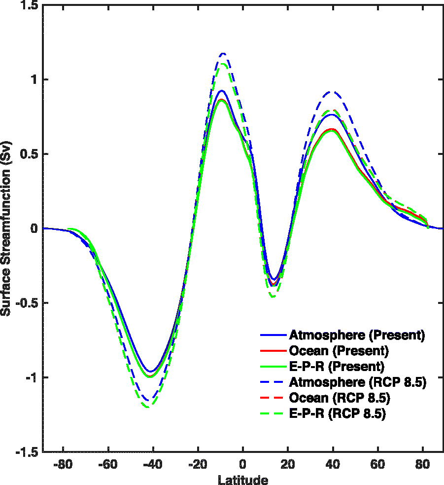
Fig. 5.
Water-mass stream function at the sea surface for the atmosphere (solid blue line), the ocean (solid red line) and surface freshwater flux (solid green line) for the present day climate. The dashed lines represent the future climate (RCP 8.5 scenario).
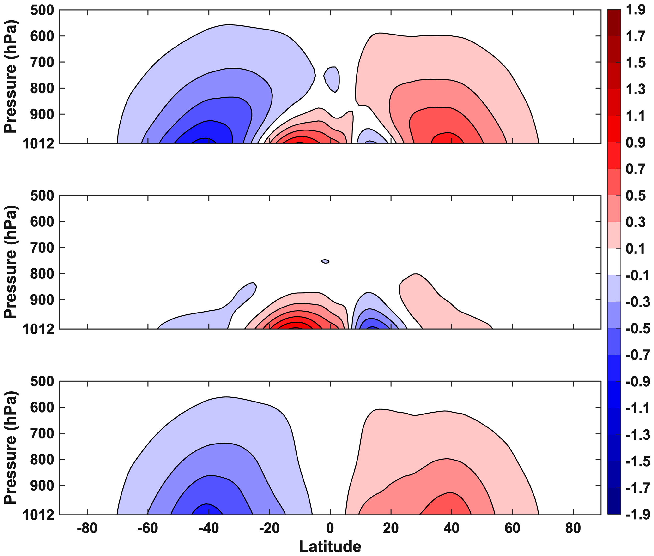
Fig. 6.
Decomposition of the atmospheric water-mass stream function (top panel) into mean-flow (middle panel) and transient eddy contribution (bottom panel). All transports are in Sv (). Red cells correspond to clockwise circulation and blue to anti-clockwise circulation.
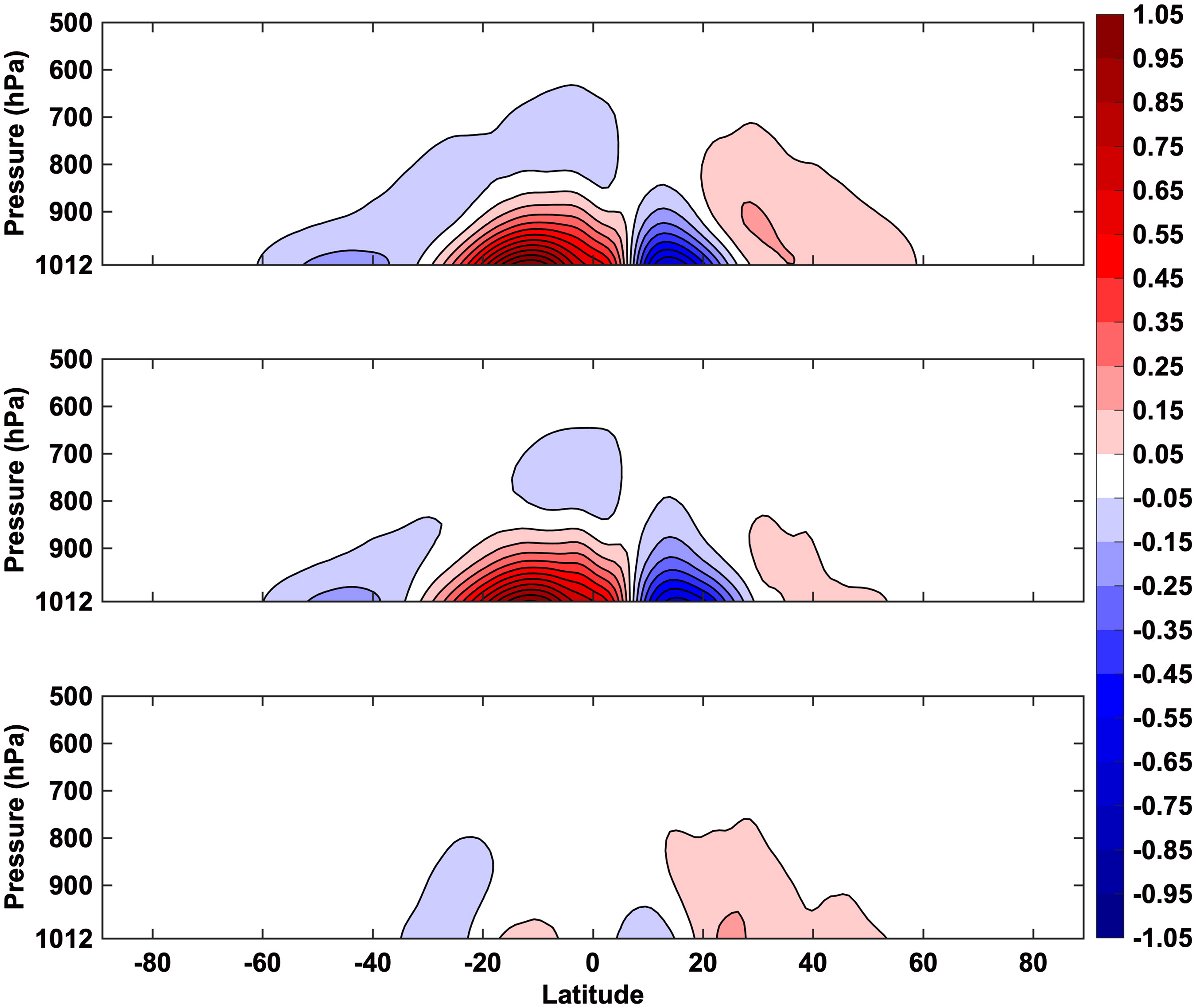
Fig. 7.
Decomposition of the mean-flow atmospheric water-mass stream function (top panel) into zonal mean flow (middle panel) and stationary eddy-zonal mean interactions contribution (bottom panel). All transports are in Sv (). The mean-flow atmospheric water-mass stream function here is the same as in Fig. 6 middle panel, but with different contour interval.
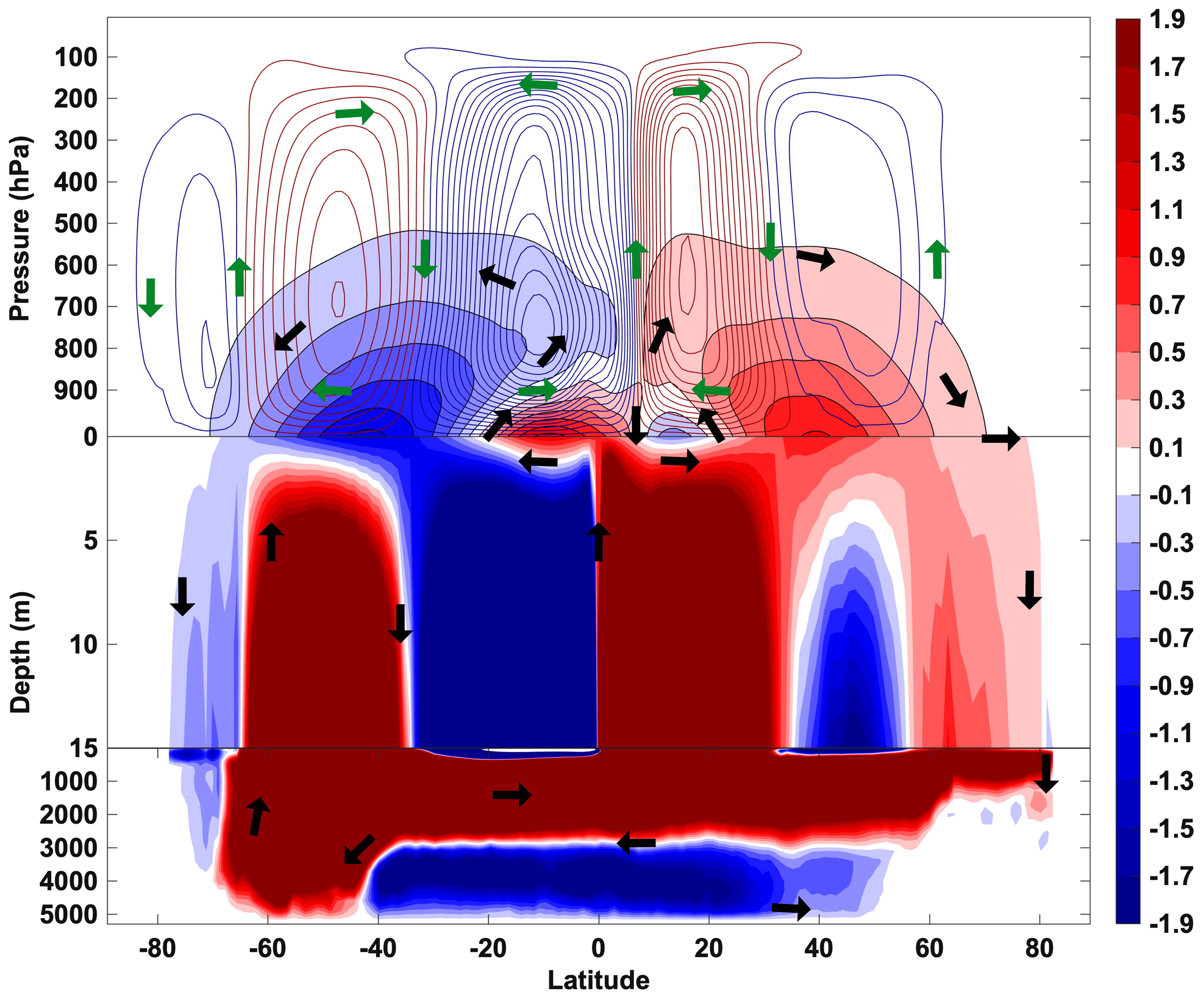
Fig. 8.
The global water-mass overturning stream function for the coupled ocean–atmosphere system superimposed with the global air-mass overturning stream function for the future climate (RCP 8.5). Black arrows shows the water-mass transport direction and green arrows indicate the air-mass transport direction. All transports are in Sv (). Note that the colour scale is saturated. Contour interval for air-mass transport is 6 Sv.