
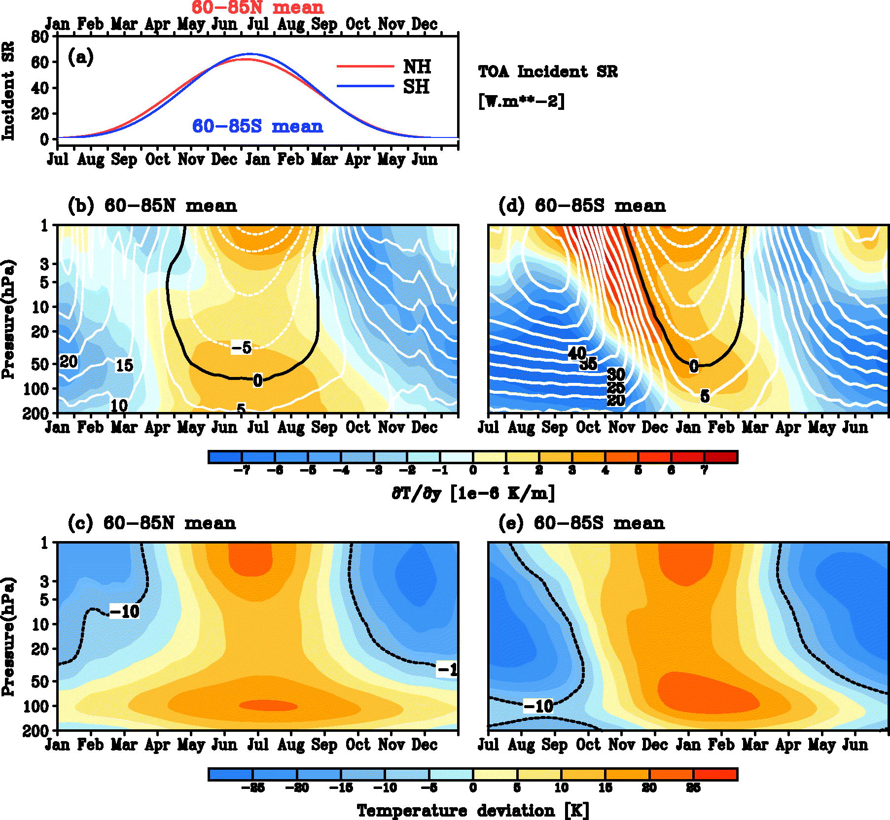
Fig. 1.
Seasonal cycle of NH and SH (a) incident solar radiation at the top of the atmosphere; (b) and (d) zonal-mean zonal wind (contour) and temperature gradient (shaded); (c) and (e) zonal-mean temperature deviations from the global mean (shaded and contour). All variables are averaged over 60–85° of NH and SH, respectively.
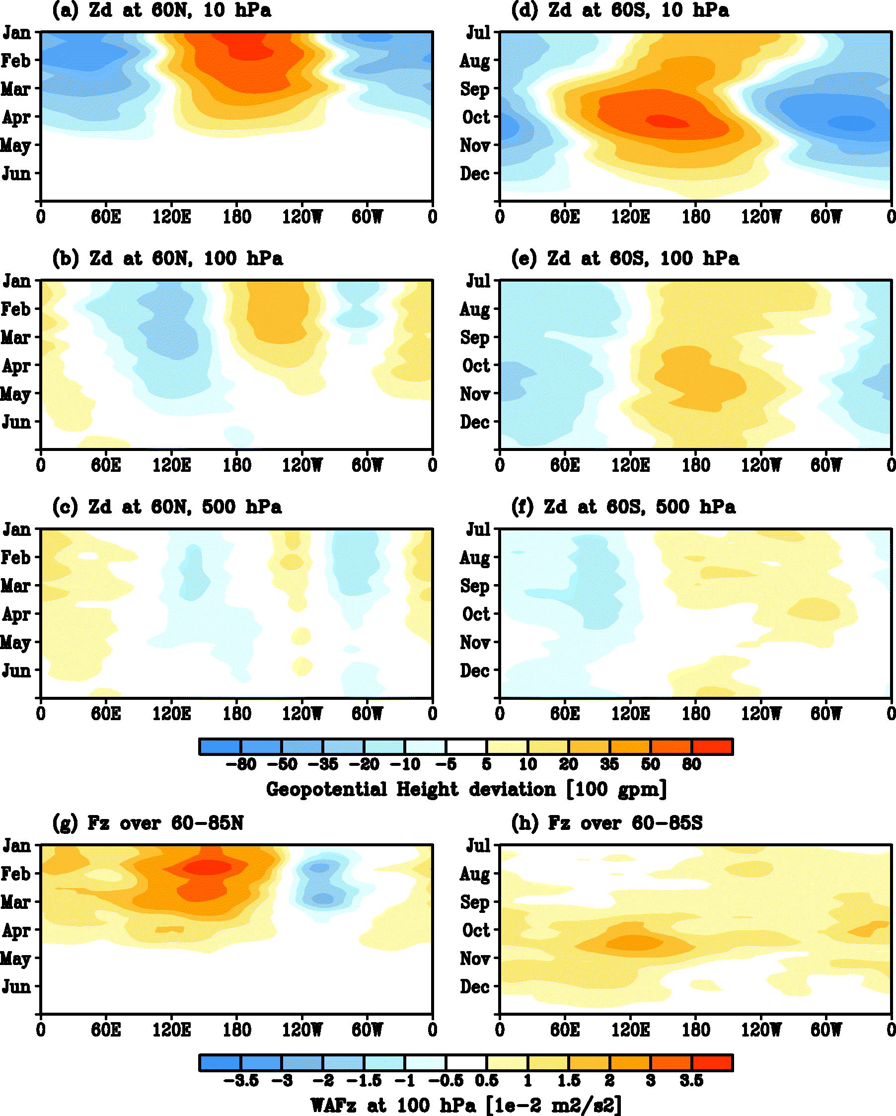
Fig. 2.
Longitude-time cross sections of geopotential height deviation from the zonal-mean for three different vertical levels at (a–c) 60°N and (d–f) 60°S, along with WAFz at 100 hPa averaged over (g) 60°N–85°N and (h) 60°S–85°S.
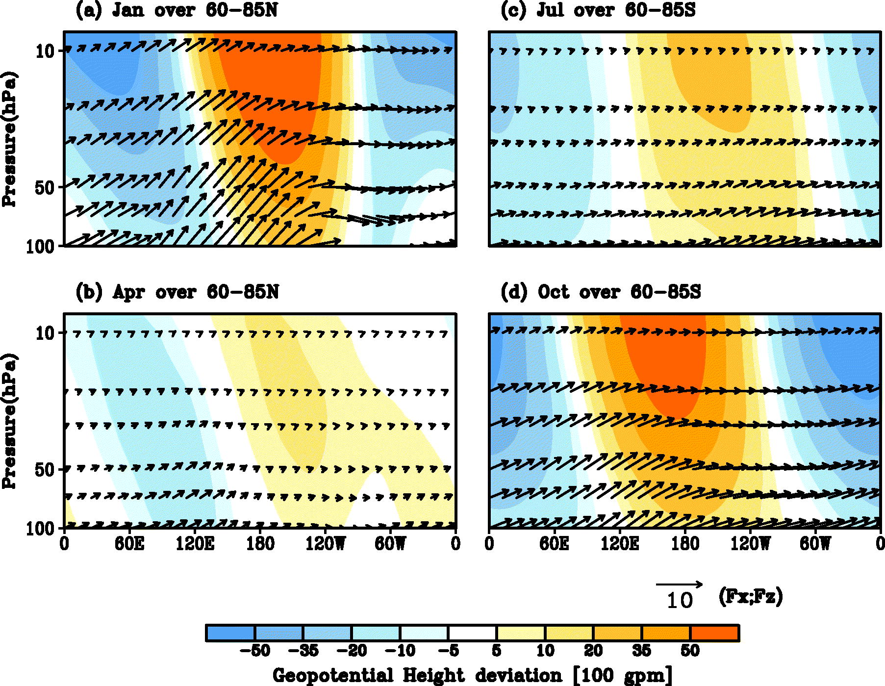
Fig. 3.
Climatology of the longitude-pressure cross sections of geopotential height deviations from the zonal-mean (shaded) and WAFs (vectors) averaged over 60°N–85°N in (a) January and (b) April, and over 60°S–85°S in (c) July and (d) October.
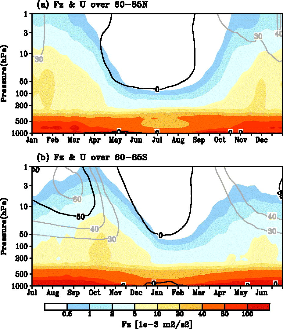
Fig. 4.
Seasonal cycle of the zonal-mean WAFz (shaded) and zonal wind (contour, zonal winds equal zero and greater than 30 m/s are shown) in the atmosphere over (a) 60°N–85°N and (b) 60°S–85°S.
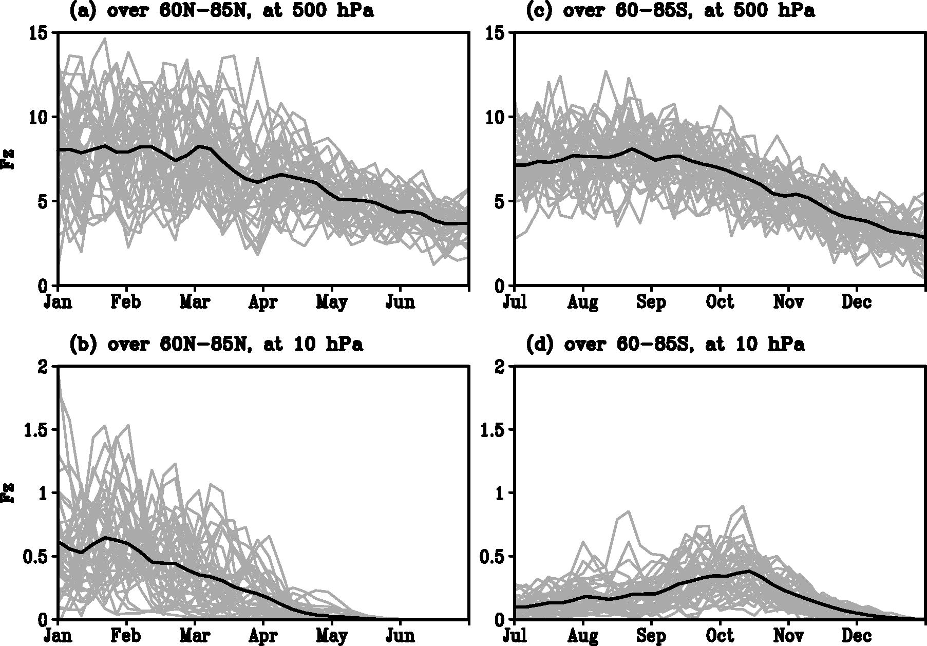
Fig. 5.
Interannual variability of the evolutions of zonal-mean WAFz from winter to summer at 500 hPa (a, c) and 10 hPa (b, d), averaged over 60°N–85°N (a, b) and 60°S–85°S (c, d). Grey lines are for the years 1979–2016. The black line is for the long-term mean. Unit: 10−2m2s−2.
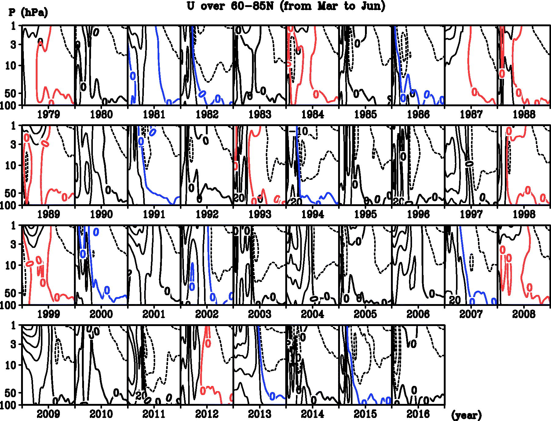
Fig. 6.
Evolutions of stratospheric zonal-mean zonal wind over 60°N–85°N from March to June each year for the period 1979–2016. Contour interval is 10 m/s. The zero-contour line is shown in red or blue depending, respectively, on whether the transition is ‘extremely’ synchronous or asynchronous.
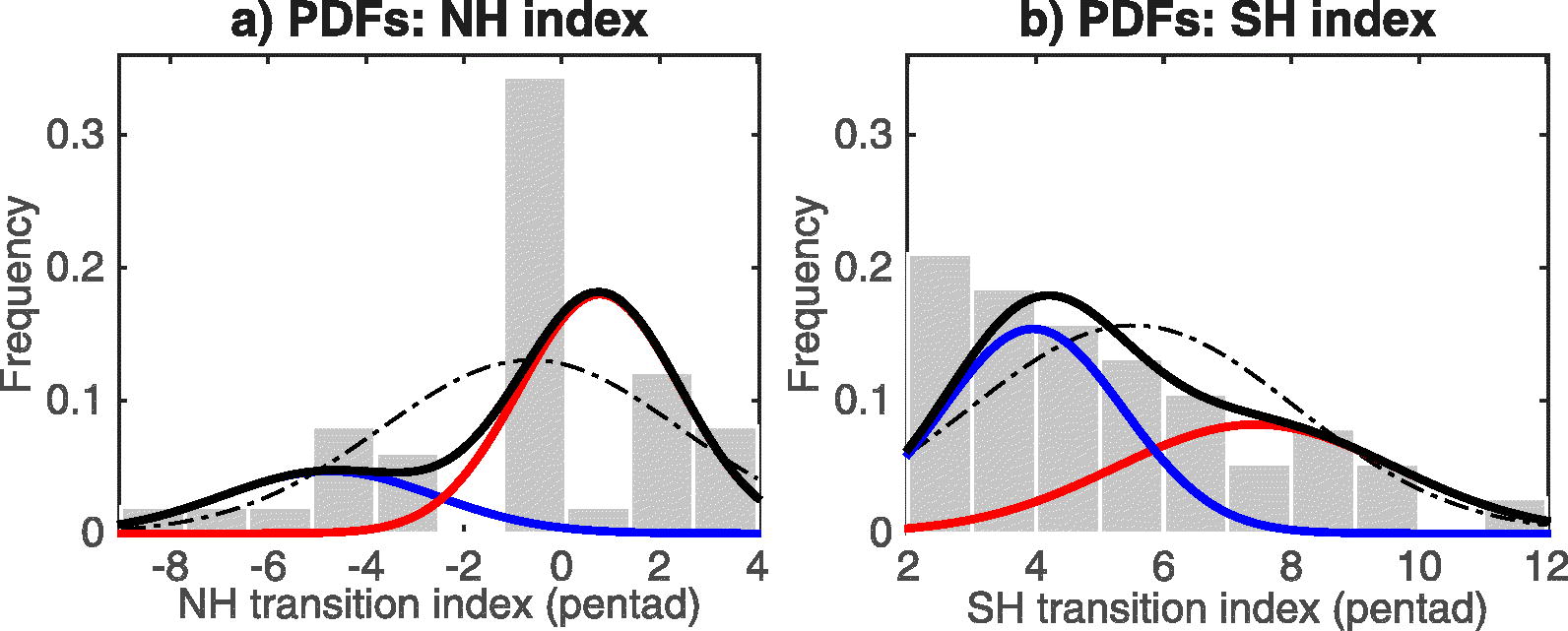
Fig. 7.
Histogram (shaded) and kernel PDF estimates of the transition indexes (black solid) for the NH (a) and SH (b). The two Gaussian components of the mixture model (see text) are shown and reflect the NH synchronous (blue)/asynchronous (red) transitions in (a); and SH steep (blue)/moderate (red) transitions in (b). The Gaussian PDFs fitted to the data are also shown (dash-dot).
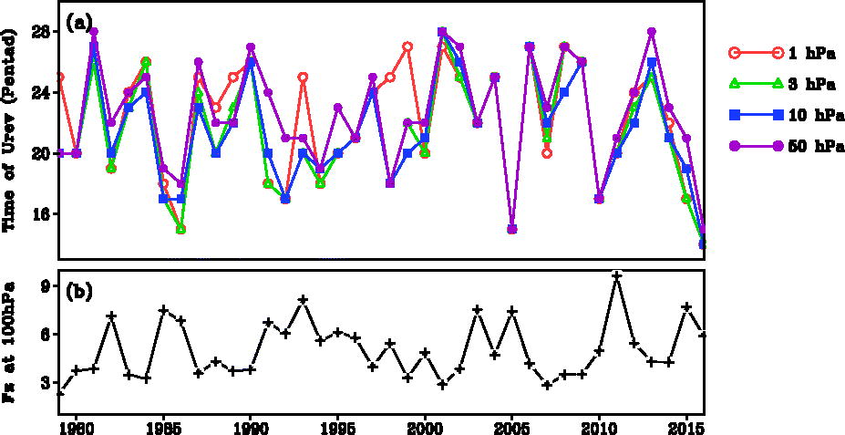
Fig. 8.
Interannual variations of (a) the seasonal transition pentads at 1 hPa (red), 3 hPa (green), 10 hPa (blue) and 50 hPa (purple); and (b) spring mean of WAFz from pentads 13 to 28 at 100 hPa. Units: (a) pentads, and (b) 10−3 m2/s2.
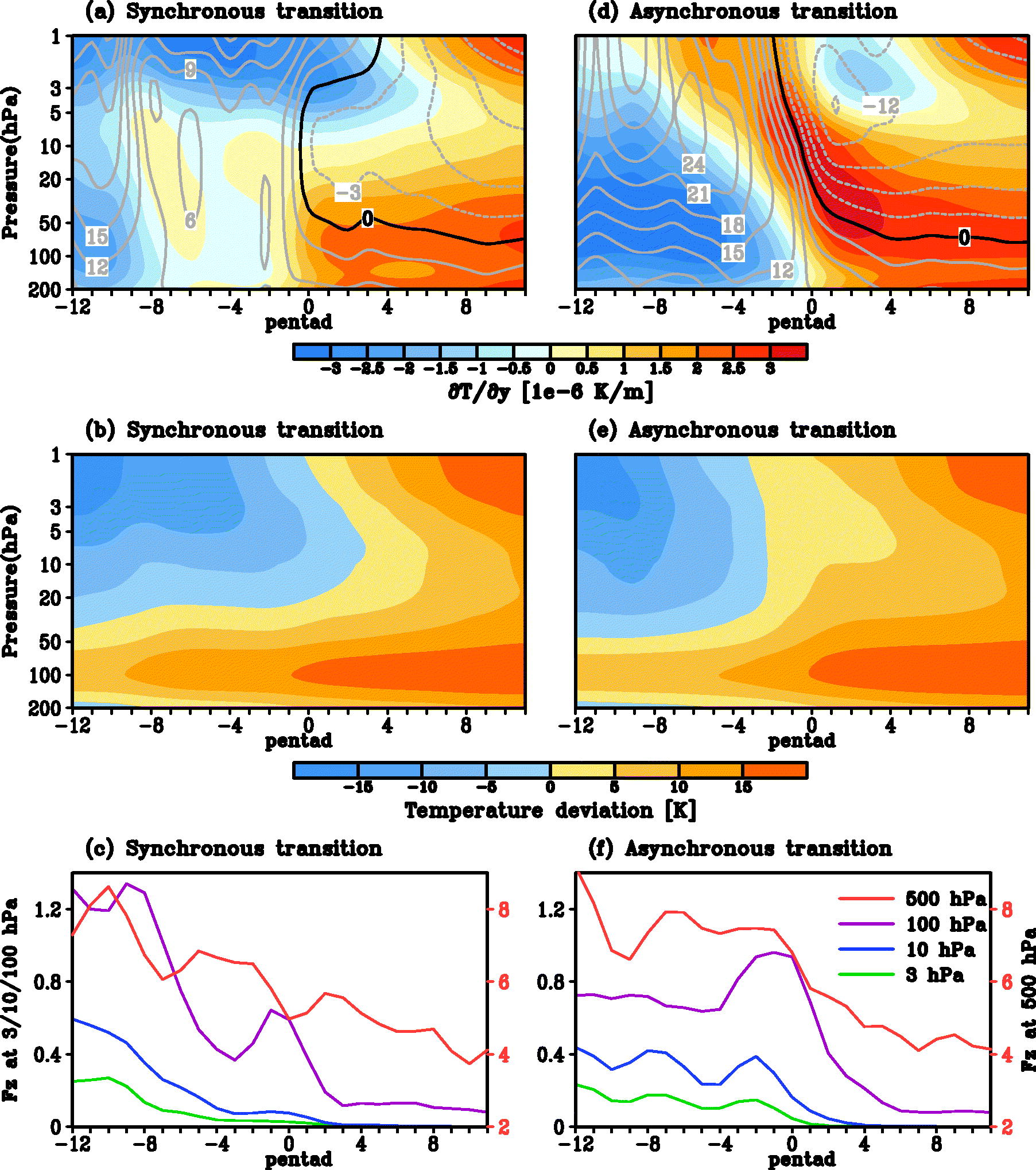
Fig. 9.
Temporal evolutions during synchronous (a–c) and asynchronous (d–f) years of zonal-mean averaged over 60°N–85°N of (a and d) temperature gradient (shaded) and zonal wind (contour, in m/s), (b and e) temperature deviation from the global mean, and (c and f) upward wave activity fluxes, based on a composite analysis of 10 extreme years. Units on the horizontal axis are in pentads relative to the reference pentad.
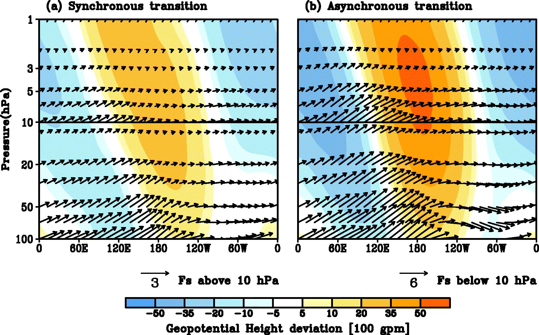
Fig. 10.
The Longitude-pressure cross sections of 9-pentad prior to the transition pentad mean geopotential height deviations from the zonal mean (shaded) and WAFs (vectors) averaged over 60°N–85°N composite in (a) synchronous, and (b) asynchronous cases. Units of WAFs, m2/s2.
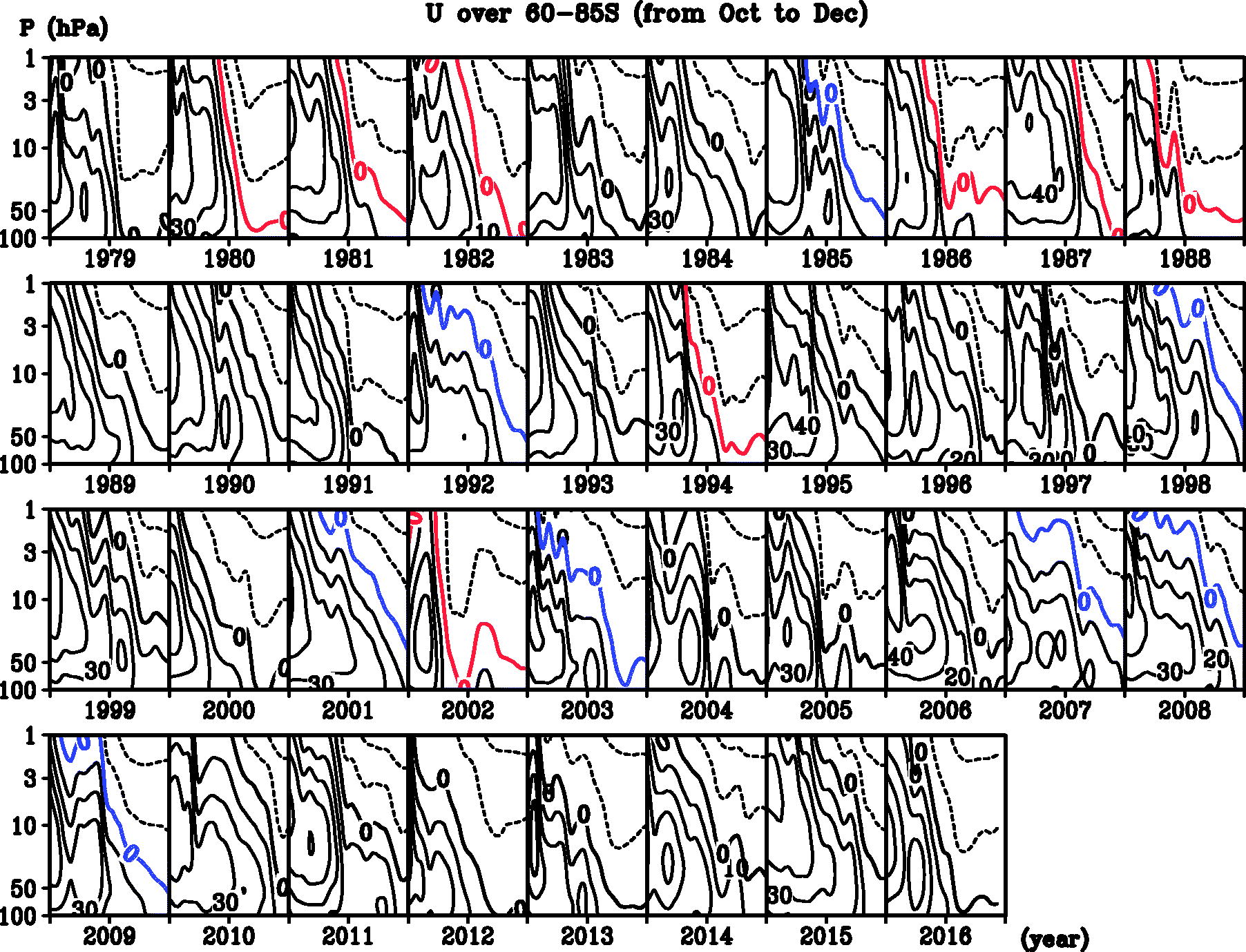
Fig. 11.
Evolutions of stratospheric zonal-mean zonal wind over 60°S–85°S from October to December each year for the period 1979–2016. Contour interval is 10 m/s. The zero-contour line is shown in red or blue depending, respectively, on whether the transition is ‘extremely’ steep or moderate.
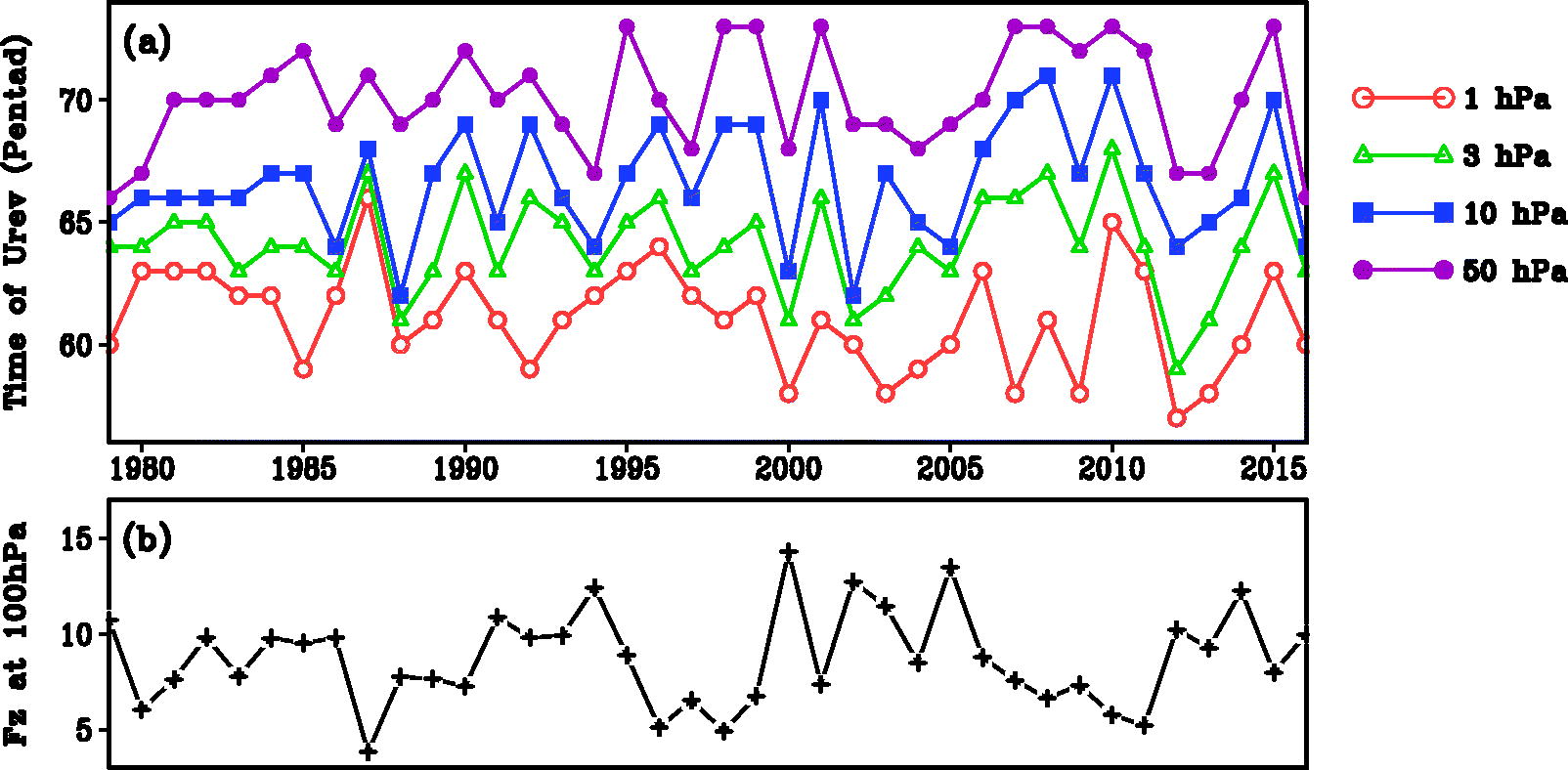
Fig. 12.
Interannual variations of (a) the seasonal transition pentads at 1 hPa (red), 3 hPa (green), 10 hPa (blue) and 50 hPa (purple); and (b) spring mean of WAFz. Units: (a) pentads, and (b) 10−3 m2/s2.
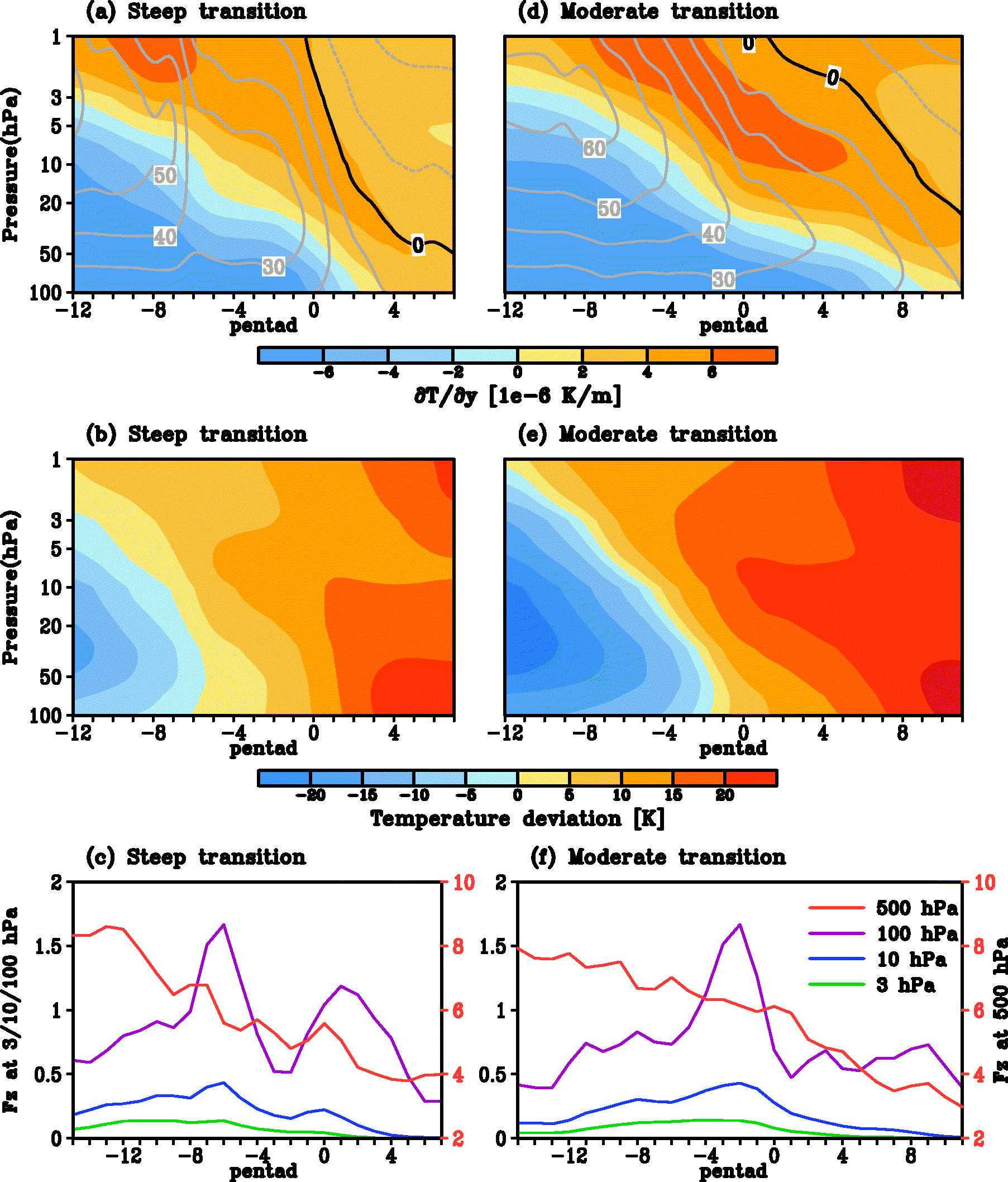
Fig. 13.
Temporal evolutions during steep (a–c) and moderate (d–f) years of zonal-mean averaged over 60°S–85°S of (a and d) temperature gradient (shaded) and zonal wind (contour, in m/s), (b and e) temperature deviation from the global mean, and (c and f) upward wave activity fluxes, based on a composite analysis of 8 extreme years. Units on the horizontal axis are in pentads relative to the reference pentad.
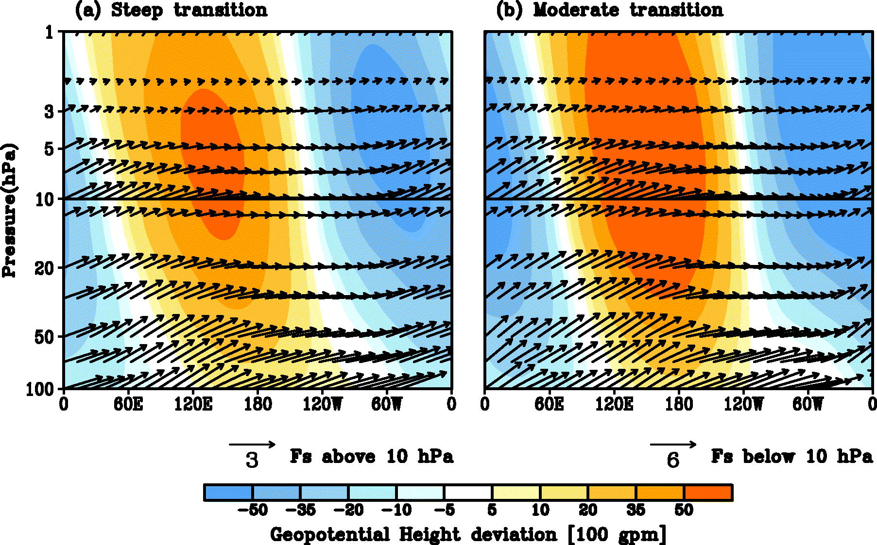
Fig. 14.
The Longitude-pressure cross sections of 9-pentad prior to the transition pentad mean geopotential height deviations from the zonal mean (shaded) and WAFs (vectors) averaged over 60°N–85°S composite in (a) steep, and (b) moderate cases. Units of WAFs, m2/s2.