
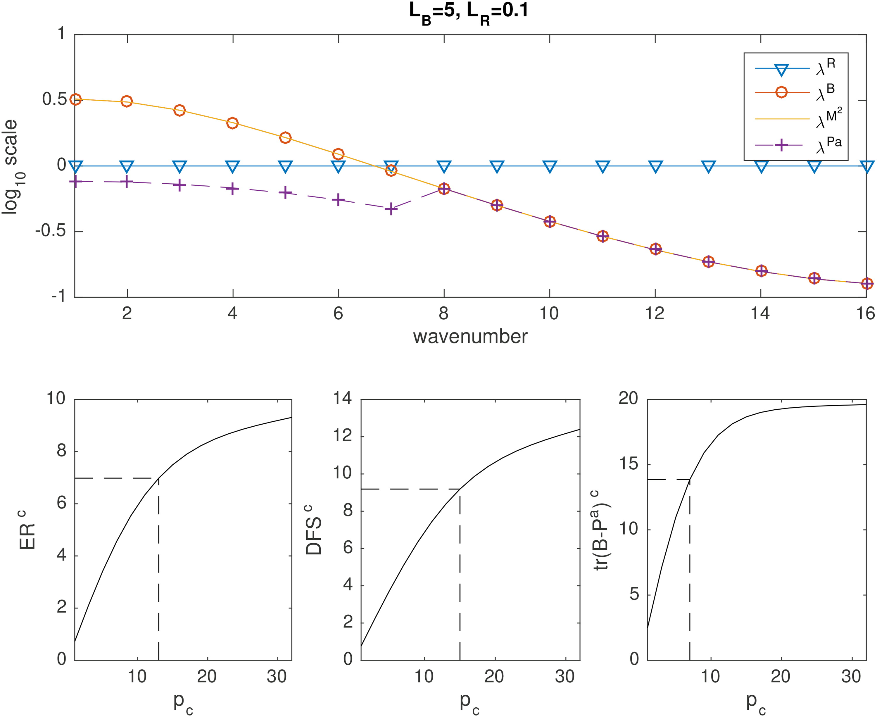
Fig. 1.
Top: Eigenvalues of (20) (yellow line), (blue triangles) and (red circles) for the case of SOAR correlation functions with and Also plotted are the eigenvalues of (purple crosses) when compressed observations retaining 75% of the total ER are assimilated (13 compressed observations in this case). Bottom: (left), (middle) and (right) as a function of the number of compressed observations ordered according to the eigenvalues of The dashed lines indicate the number of compressed observations needed to achieve 75% of the total value. These numbers are also given in Table 1.
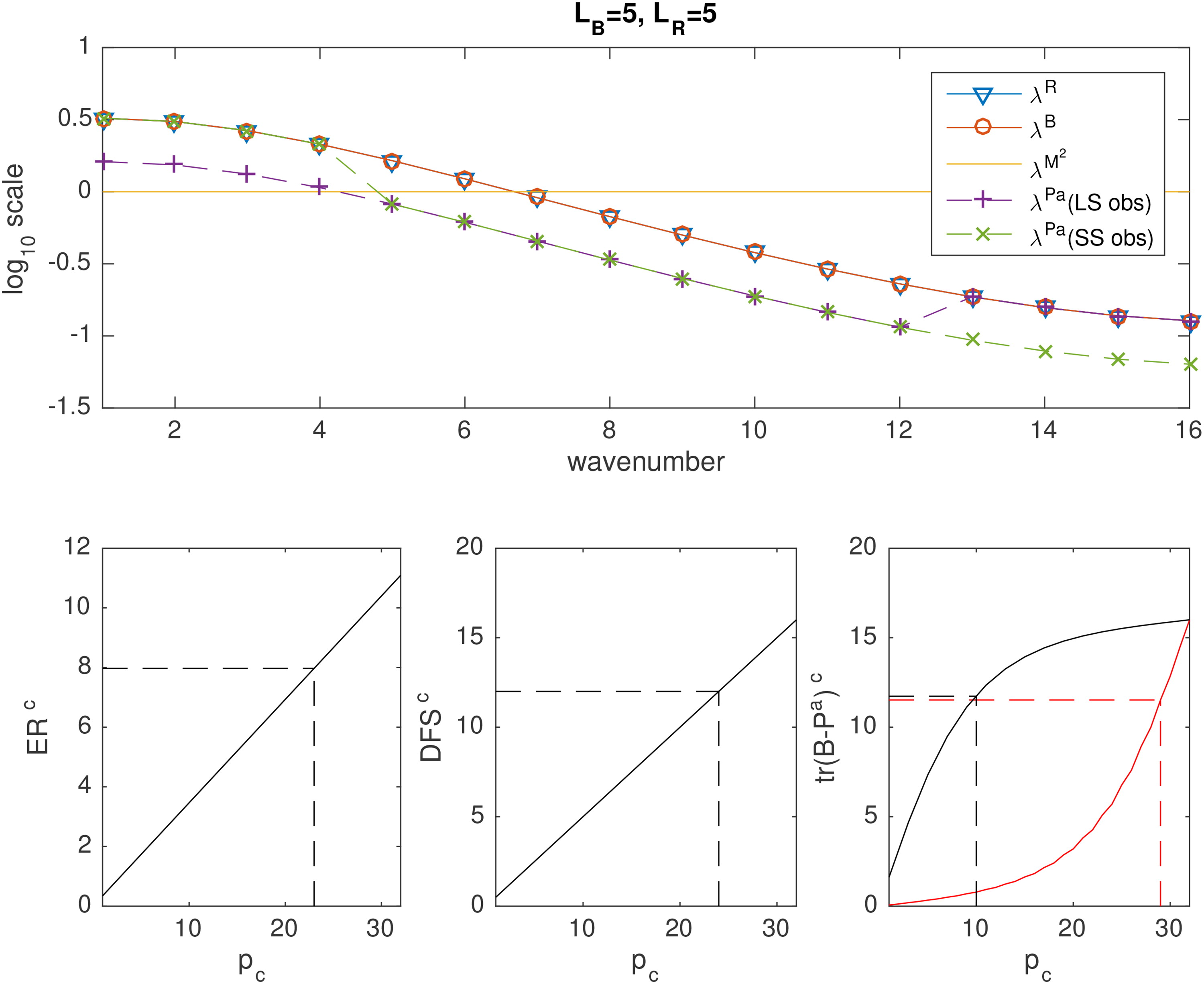
Fig. 2.
As in Fig. 1 but for The black line of the last panel shows as a function of the number of compressed observations when the assimilation is performed using large-scale observations first, and the red line when the assimilation is performed using small-scale observations first.
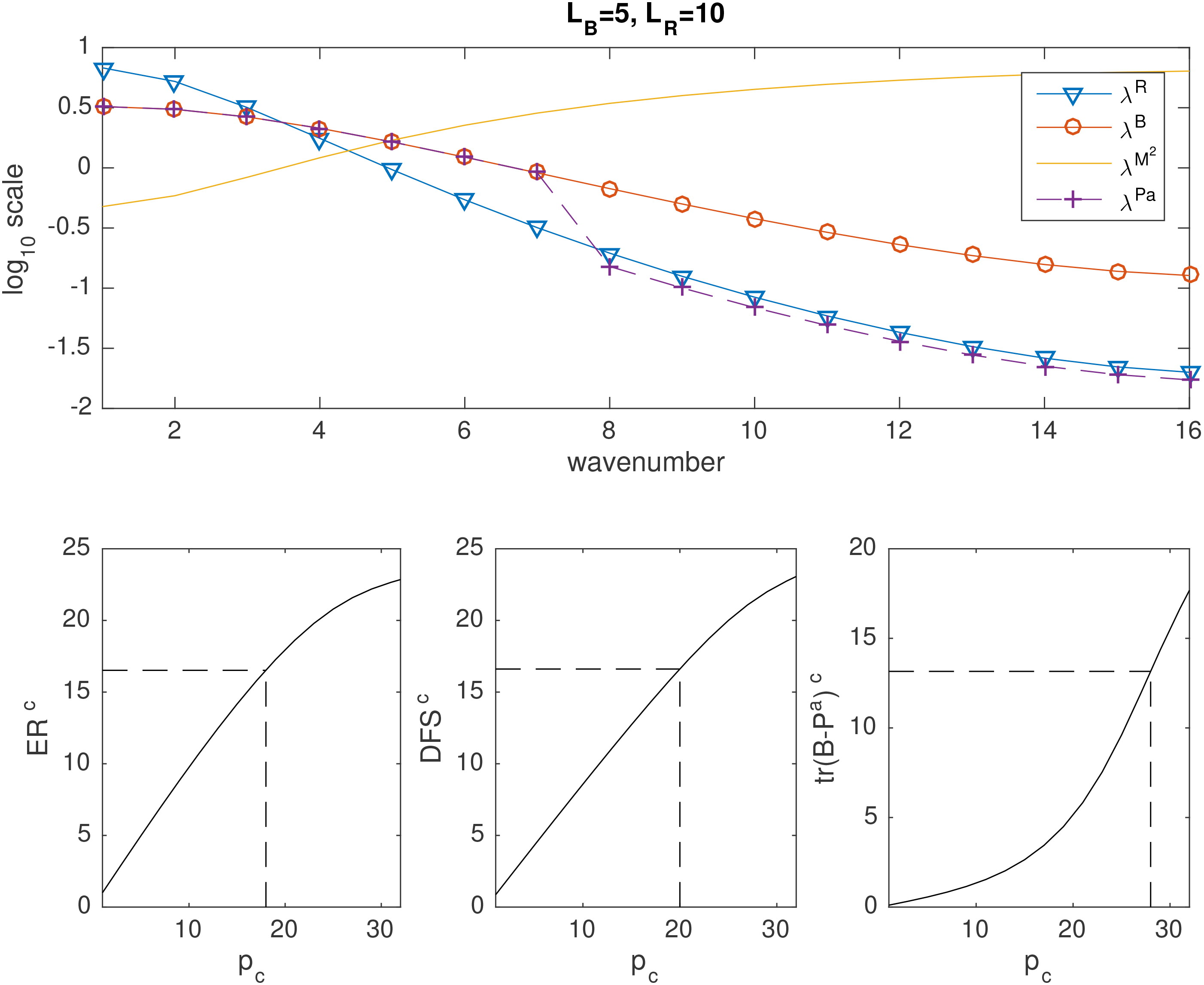
Fig. 3.
As in Fig. 1 but for
Table 1.
75% of the value of ER, DFS, and when all observations are assimilated for different values of In brackets are the number of compressed observations need to achieve these values.
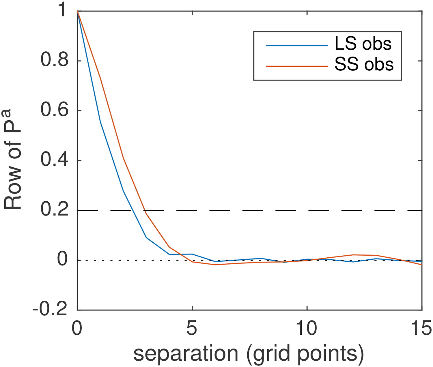
Fig. 4.
Analysis error correlation structure for the case illustrated in Fig. 2. The number of compressed observations assimilated are chosen to conserve 75% of ER. Blue: compressed observations favour large scales and red: compressed observations favour small scales.
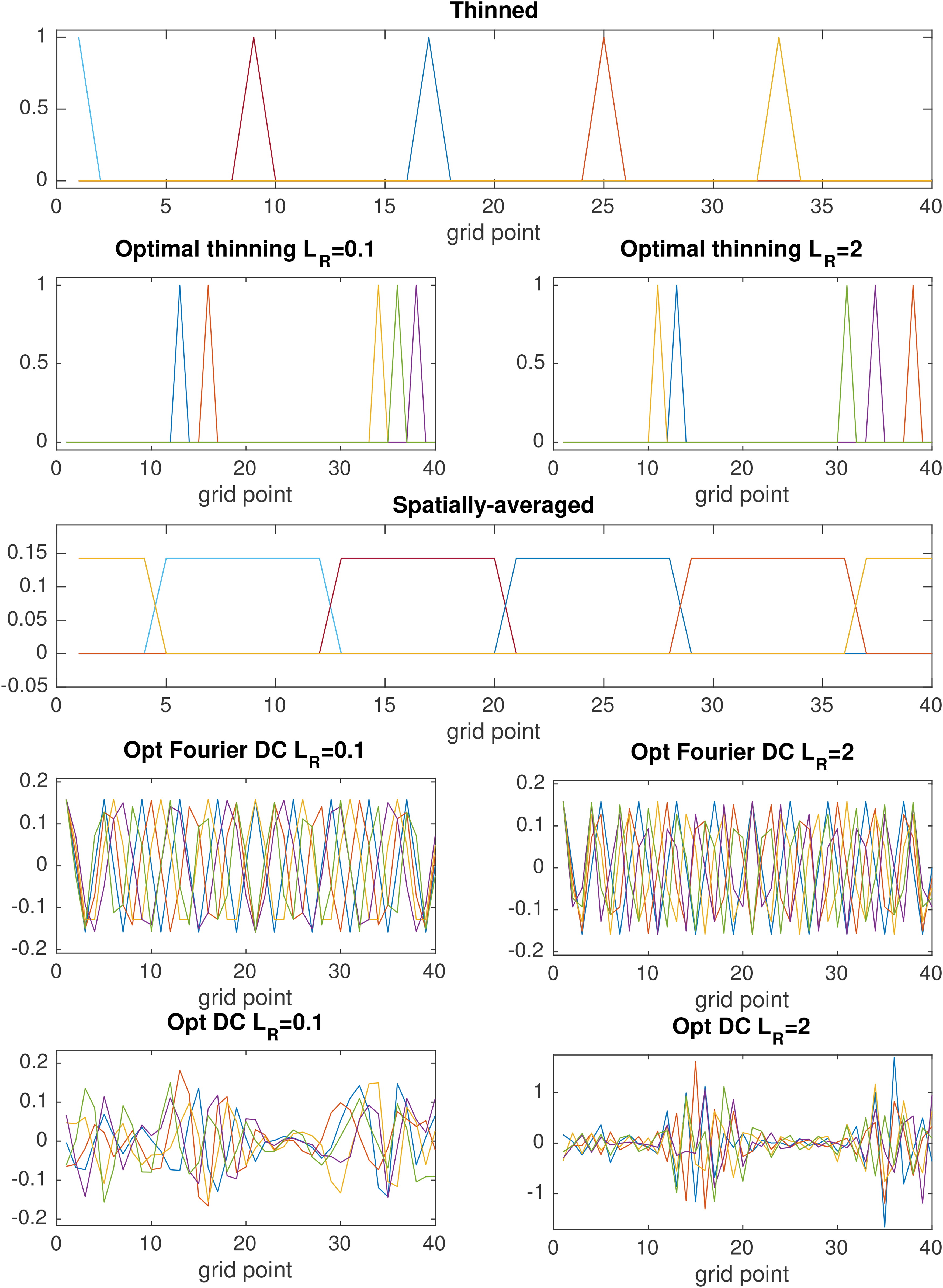
Fig. 5.
Rows of the observation operator matrix for the five strategies for reducing the observation data detailed in Section 4. The optimal strategies are illustrated for the first observation time.
Table 2.
The wave-numbers selected by the optimal Fourier data compression method at each observation time for the two different types of observations. The first observation time corresponds to the observation operator plotted in Fig. 5.
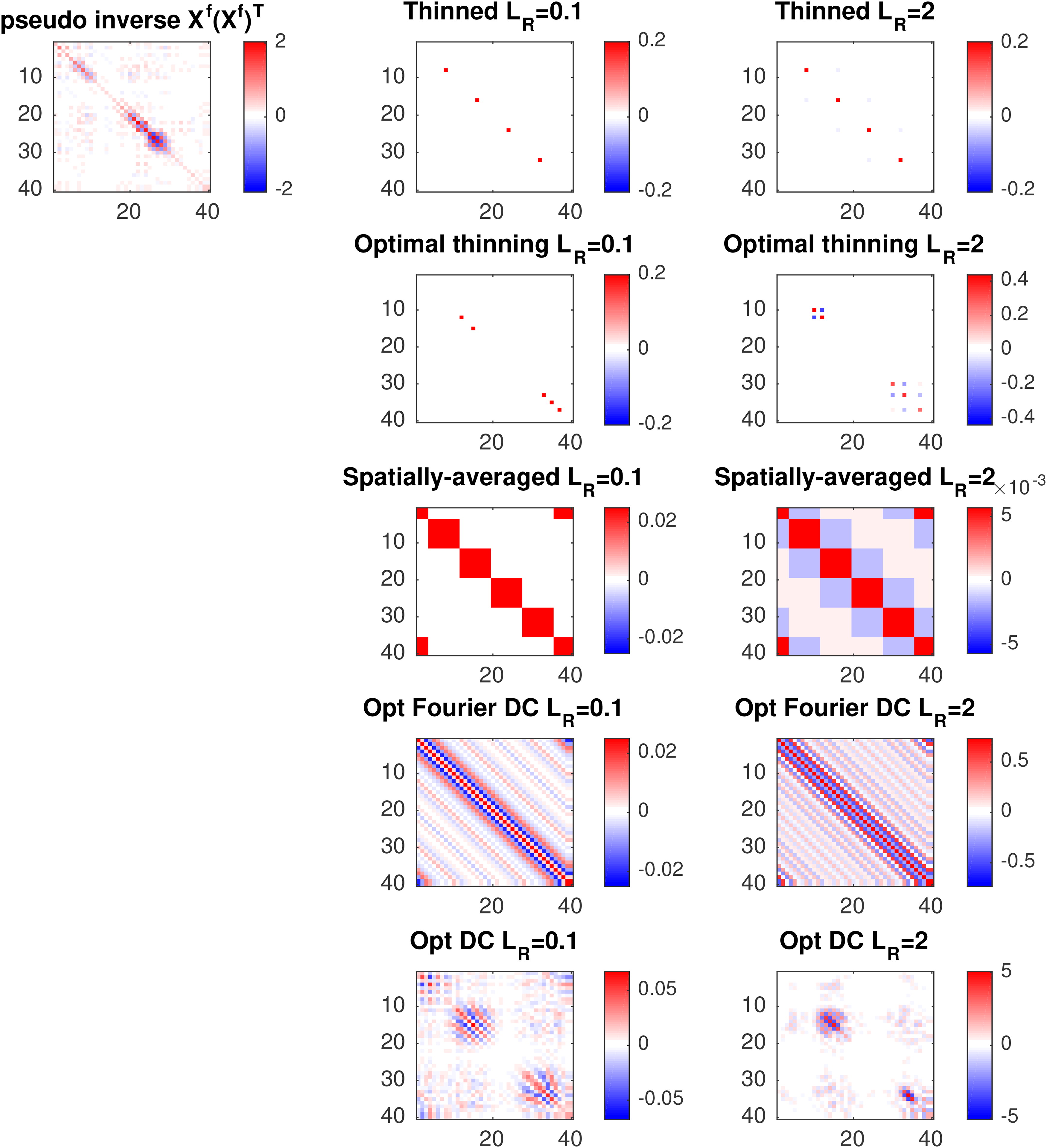
Fig. 6.
Top left: pseudo inverse of illustrated for the first observation time. Other panels: (the accuracy of the compressed observation in state space) for the 5 different thinning strategies when observation errors are uncorrelated (middle panels) and correlated (right panels) illustrated for the first observation time.
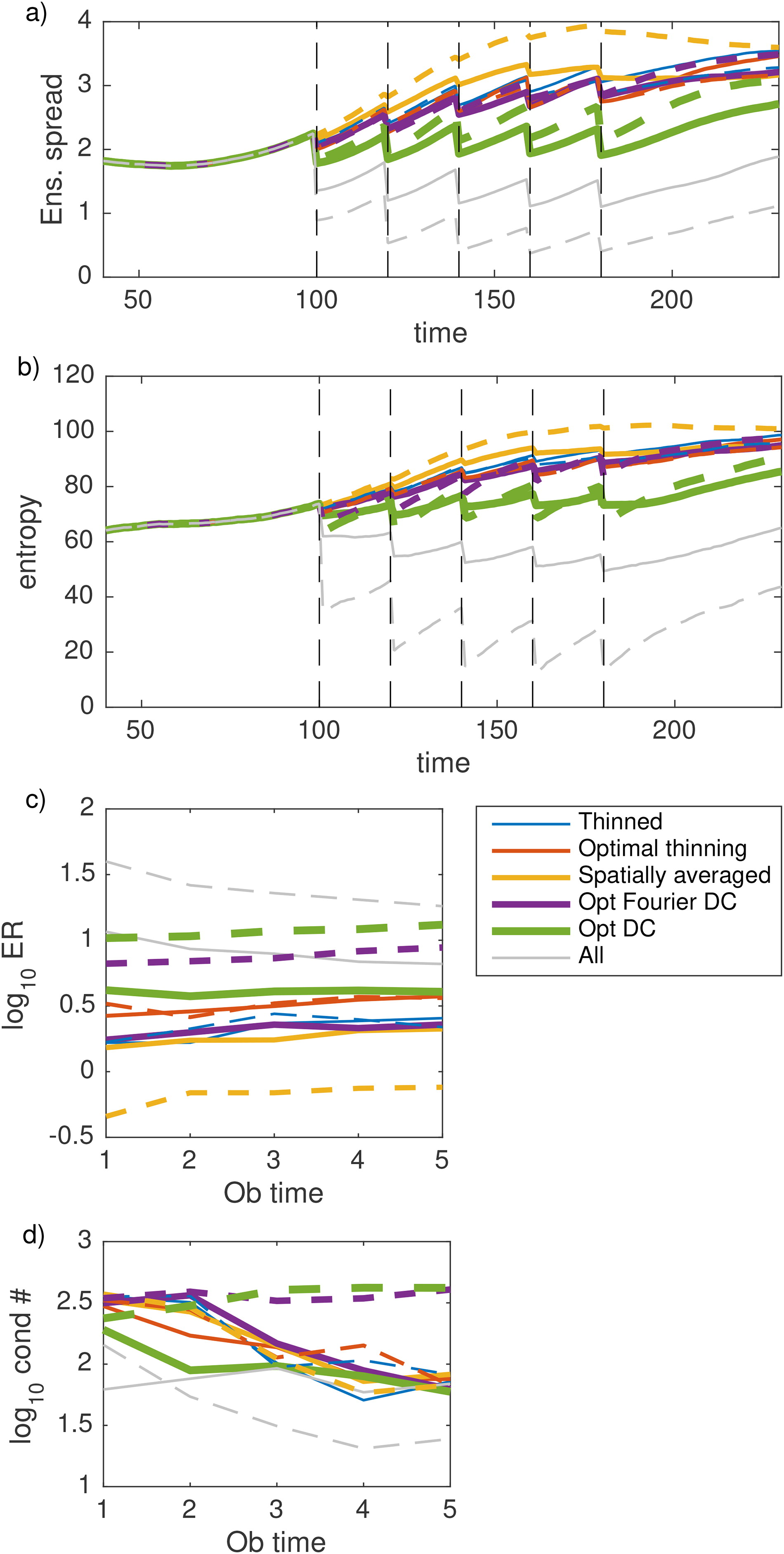
Fig. 7.
(a) Ensemble spread, (b) entropy computed using the ensemble estimate of (11), (c) and (d) log10 of the condition number of the analysis error covariance matrix for the five different thinning strategies detailed in Section 3.1. Solid lines represent results when the observation errors are uncorrelated, dashed lines represent results when the observation errors are correlated. Results are averaged over 200 experiments with different realisations of the observation and model error.