
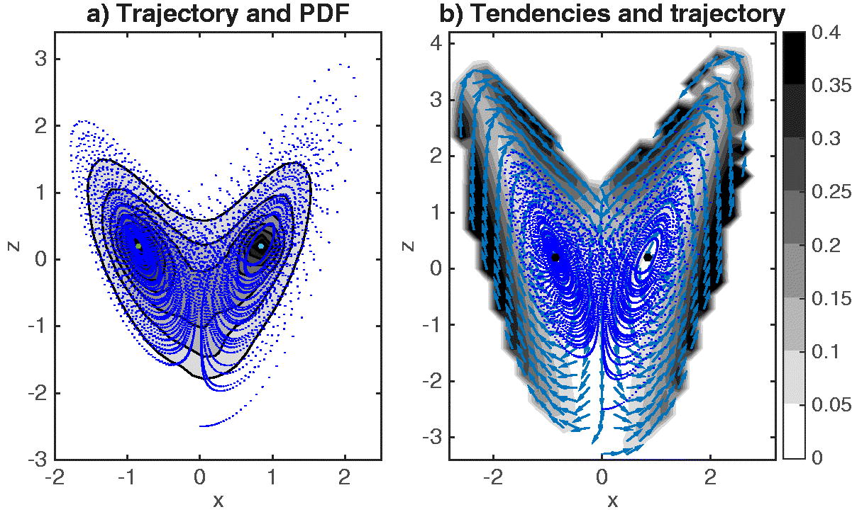
Fig. 1.
PDF of a long simulation of the Lorenz model shown by shaded and solid contours within the (x, z) plane (a), and the flow tendency within the same plane plotted in terms of magnitude (shaded) and direction (normalised vectors) within the same (x, z) plane (b). A chunk of the model trajectory is also shown in both panels along with the fixed points. Note that the variables are scaled by 10, and the value of the fixed point is subtracted from z.
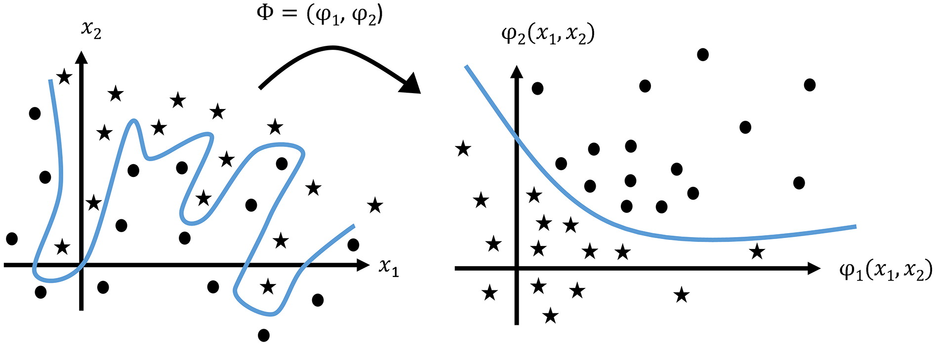
Fig. 2.
Schematic illustration of a nonlinear transformation of the system coordinates into a feature space, which permits disentanglement of the system complexity.
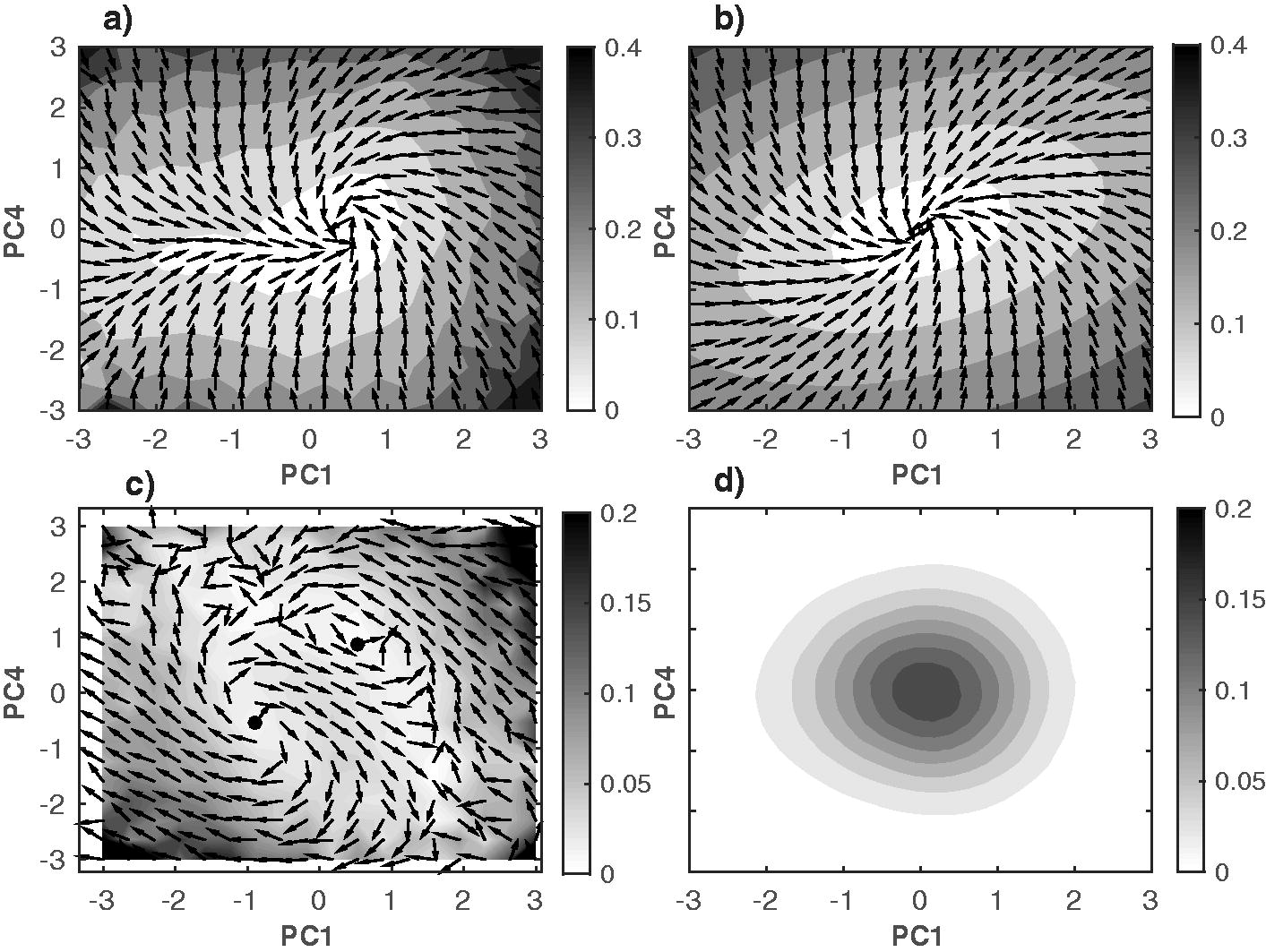
Fig. 3.
(a) Flow tendency of the mid-level streamfunction of the 3-level quasi-geostrophic model within the space spanned by PC1 and PC4 showing the normalised tendency vectors and their amplitudes. (b) The flow tendencies generated by the linear dynamics within the same state space. (c) Nonlinear component of the flow tendency obtained by subtracting (b) from (a). (d) Kernel PDF estimate of the mid-level trajectory of the 3-level model within the PC1/PC4 space.
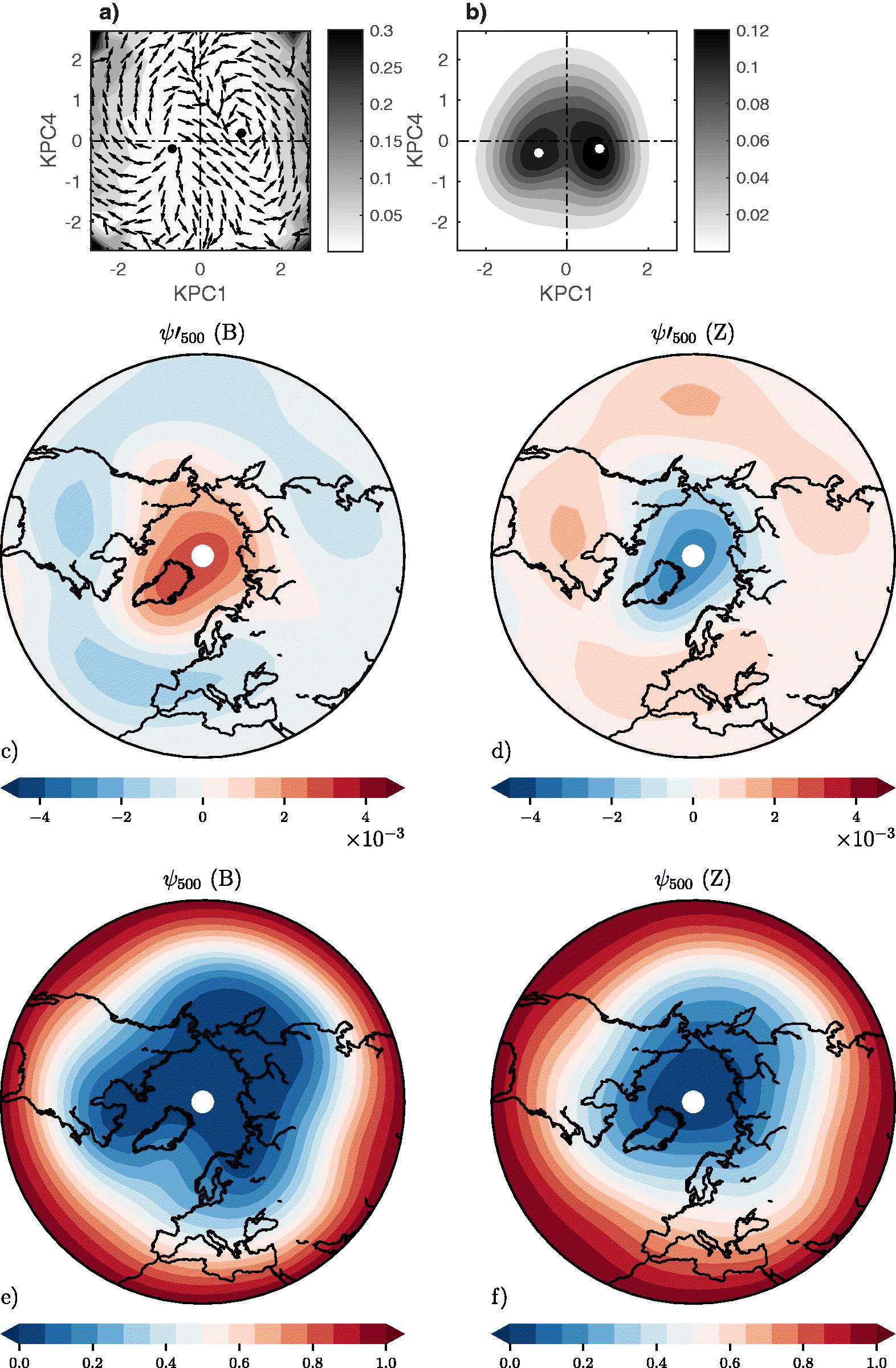
Fig. 4.
Top left: As in Fig. 3c but for the nonlinear component of the flow tendency within the space spanned by kernel PC1/PC4. Top right as in Fig. 3d but for the kernel PDF using the kernel PC1/PC4. Middle panels: The anomalous flows (or circulation regimes) of the left and right PDF modes, obtained by compositing over states within a small neighborhood of the PDF maxima. Bottom panels: total flow of the modes obtained by adding the climatology to the anomalous circulation regimes. Contour interval (middle panels) and (bottom panels).
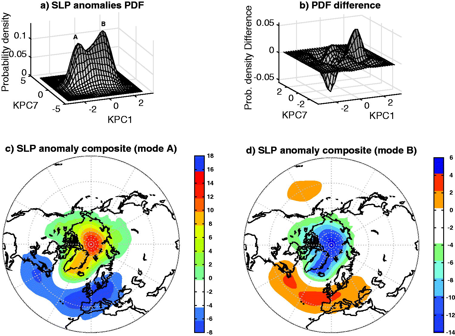
Fig. 5.
(a) Kernel PDF of the daily winter JRA-55 SLP anomalies within the kernel PC1/PC7 state space. (b) Difference between the PDFs of winter daily SLP anomalies of the first and second halves of the JRA-55 record. (c) and (d) SLP anomaly Composites over states close to the modes of the PDF of (a). Units in (c) and (d): hPa.
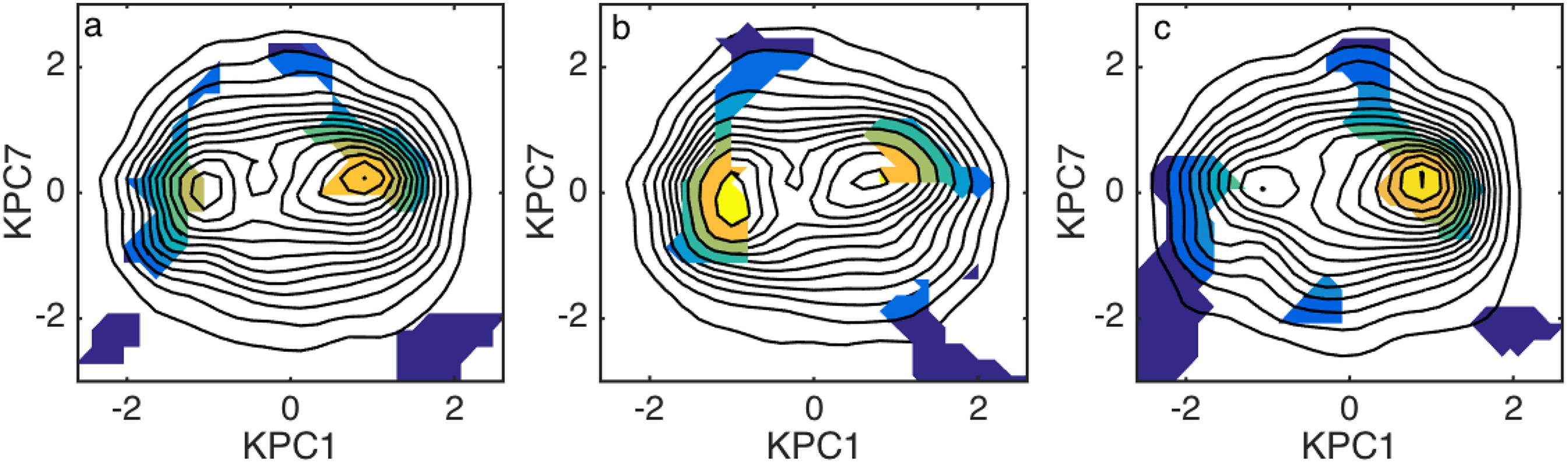
Fig. 6.
PDFs of the NH JRA-55 sea level pressure anomalies over the entire (a), the first half (b) and the second half (c) of the reanalysis period along with the 10% significance level (shading). The different colors simply refer to the PDF level and can be ignored.
Table 1.
Correlation coefficients between the 10 leading KPCs and PCs of SLP anomalies.