
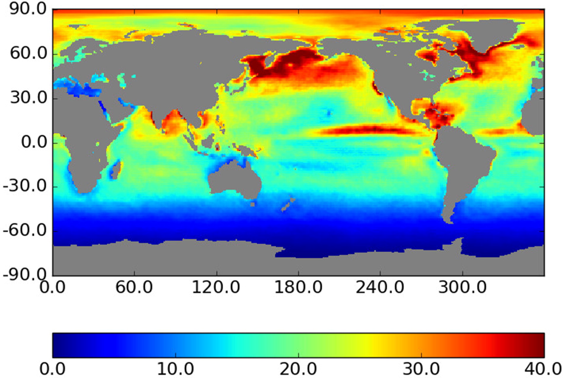
Fig. 1.
Standard deviation of the reanalysis difference for swrd in June, July and August.
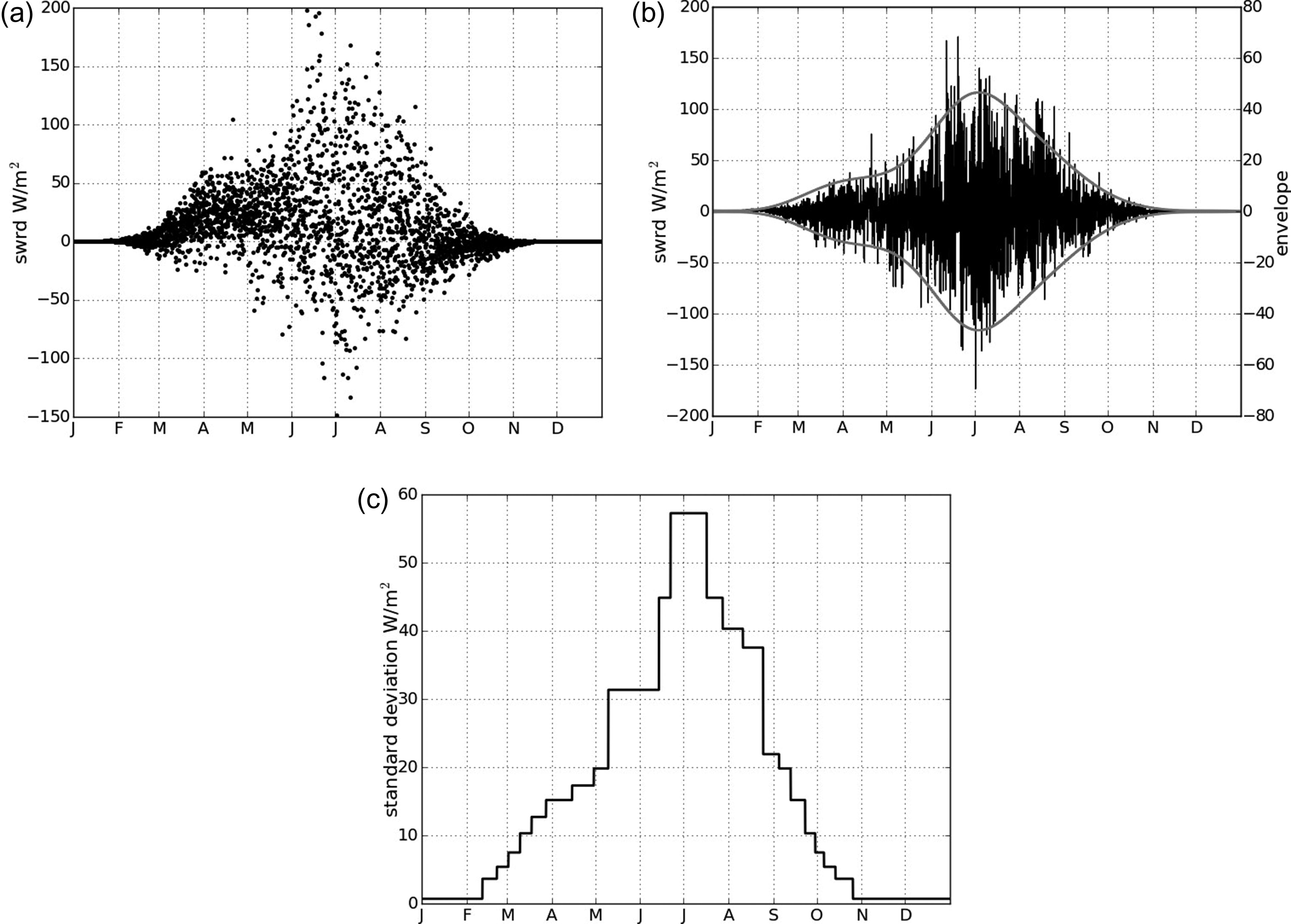
Fig. 2.
Reanalysis differences for swrd at high latitude (70N, 180E). Panel (a) shows the raw data whilst panel (b) shows the filtered data (black line; left scale) along with the wave envelope (grey line; right scale). The ten-year data is sorted by days of the year. Panel (c) represents the standard deviation calculated for the model for each time of the year.
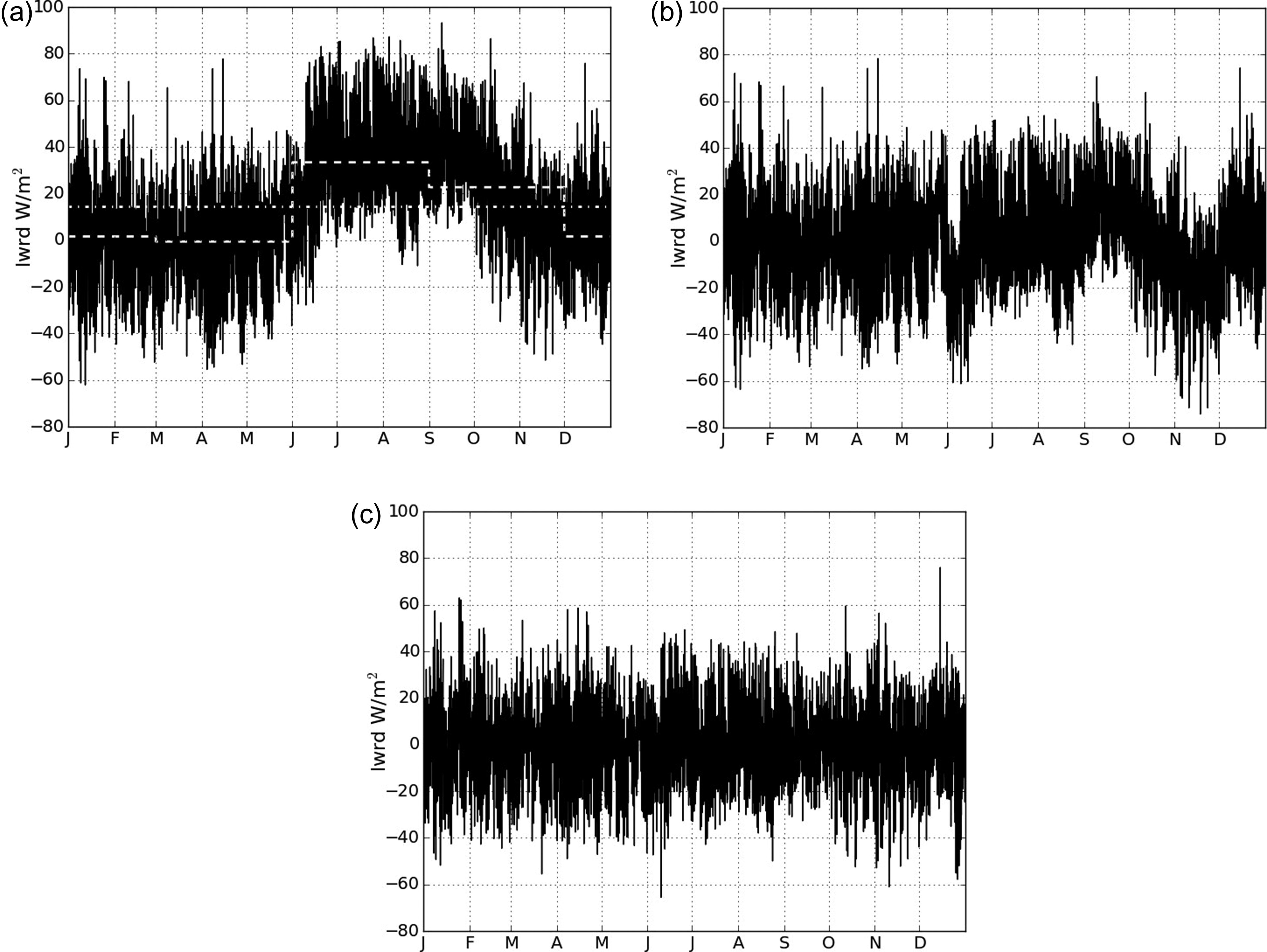
Fig. 3.
Reanalysis differences (black lines) for lwrd at high latitude (87N, 4E). In panel a, the dotted grey line and the dashed grey line represent the annual and seasonal mean, respectively. The raw data (panel a) are filtered using the seasonal mean (panel b) or a high-pass filter (panel c).
Table 1.
Sources for modelling each dependent variable. The same dependence relationships are applied for each grid point.
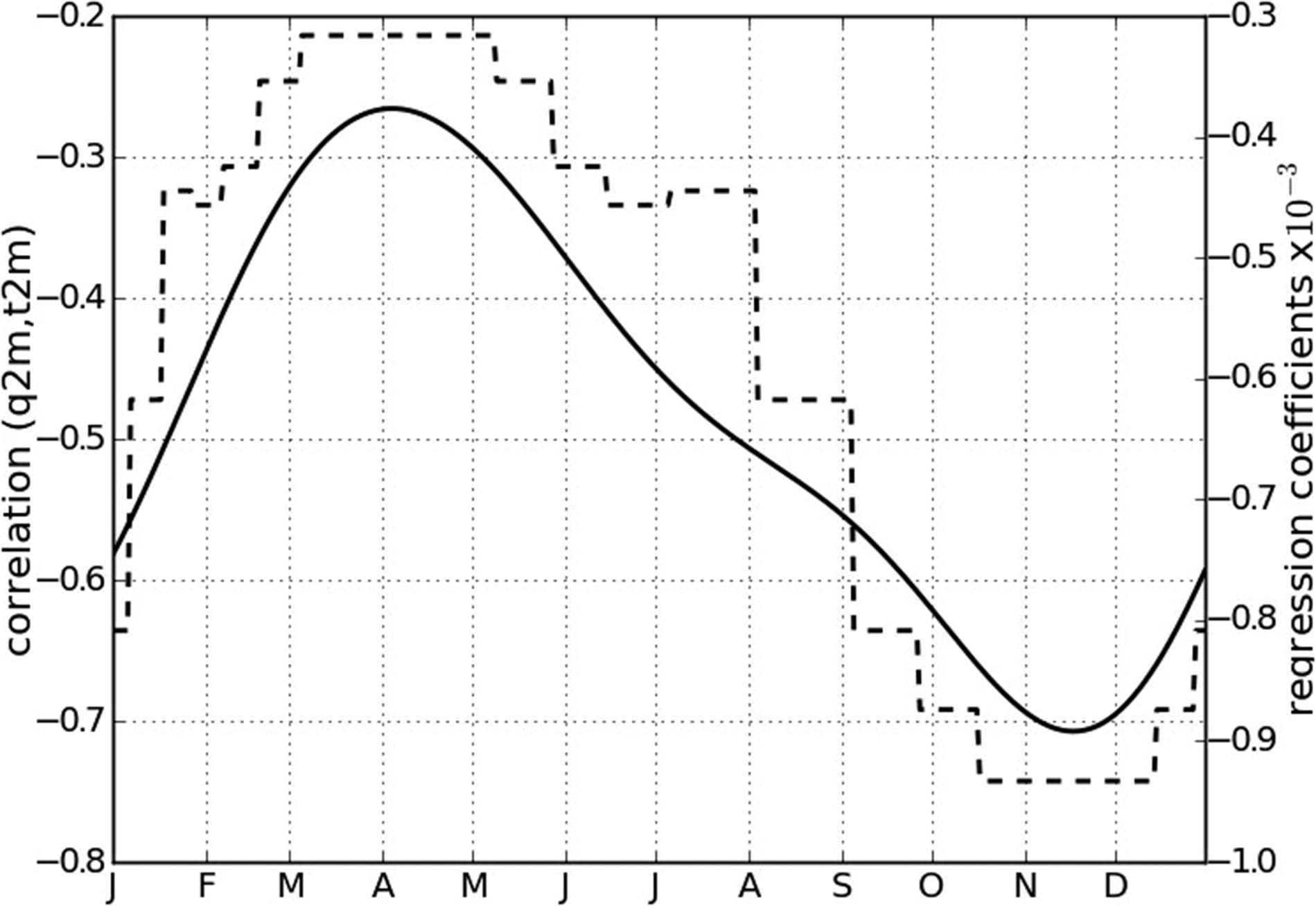
Fig. 4.
Correlation between q2m and t2m (solid line; left scale) and the resulting regression coefficient (dashed line; right scale) for q2m at 6S and 30W.
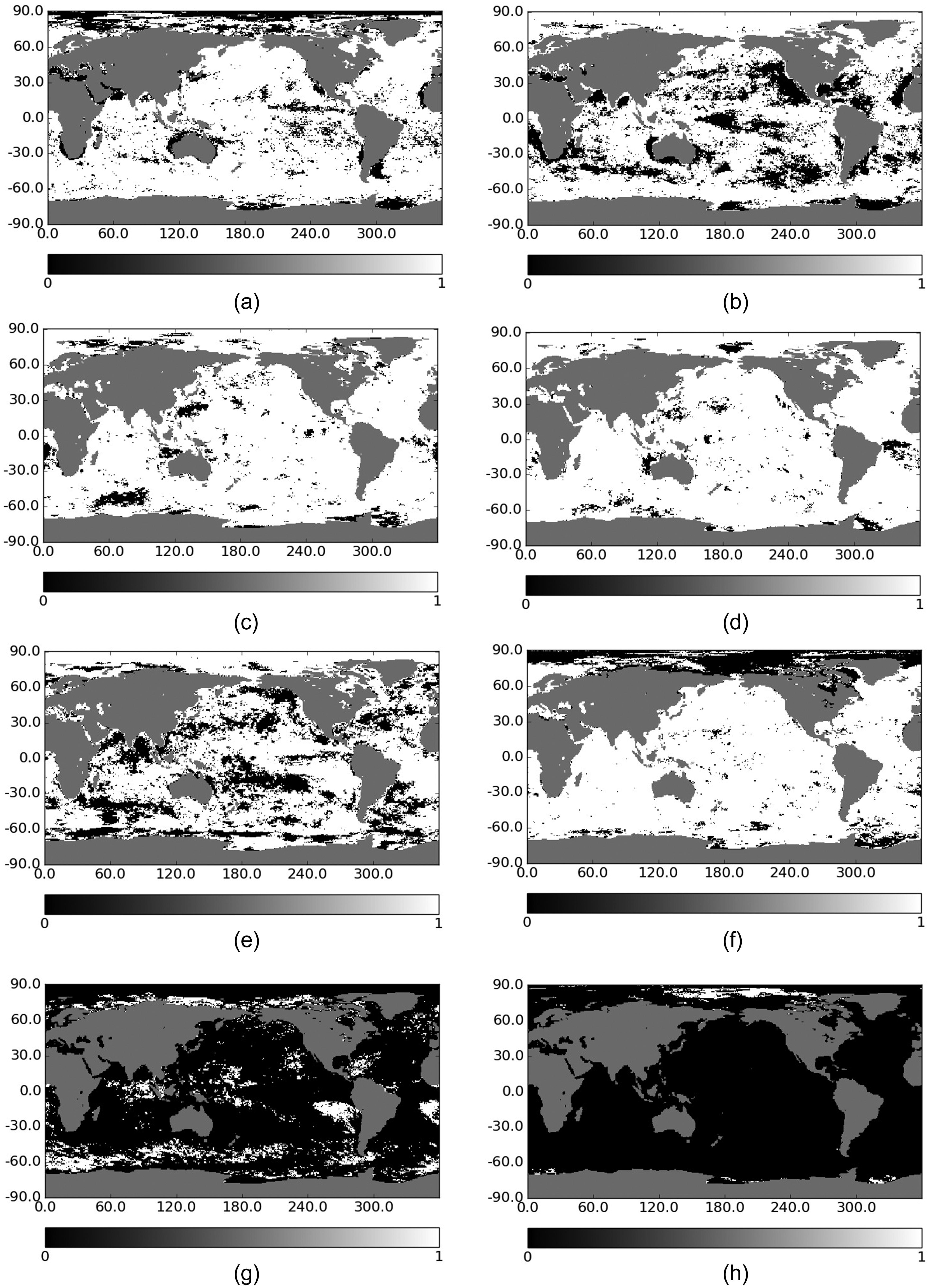
Fig. 5.
Kolmogorov-Smirnov test result with α = 5% for swrd (a), lwrd (b), u10m (c), v10m (d), t2m (e), q2m (f), precipitation (g) and snow (h). The null hypothesis is rejected for the grid points with values 0 (black), but cannot be rejected for the grid points with values 1 (white).
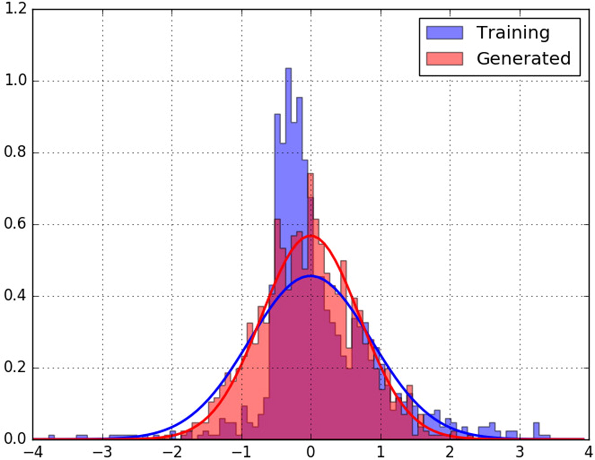
Fig. 6.
Normed histogram for the training data (blue) and the generated data (red) for swrd at high latitude (70N, 180E) from end October to mid-February. The blue and red lines represent the theoretical normal distribution associated with the standard deviation of the training and generated data, respectively.
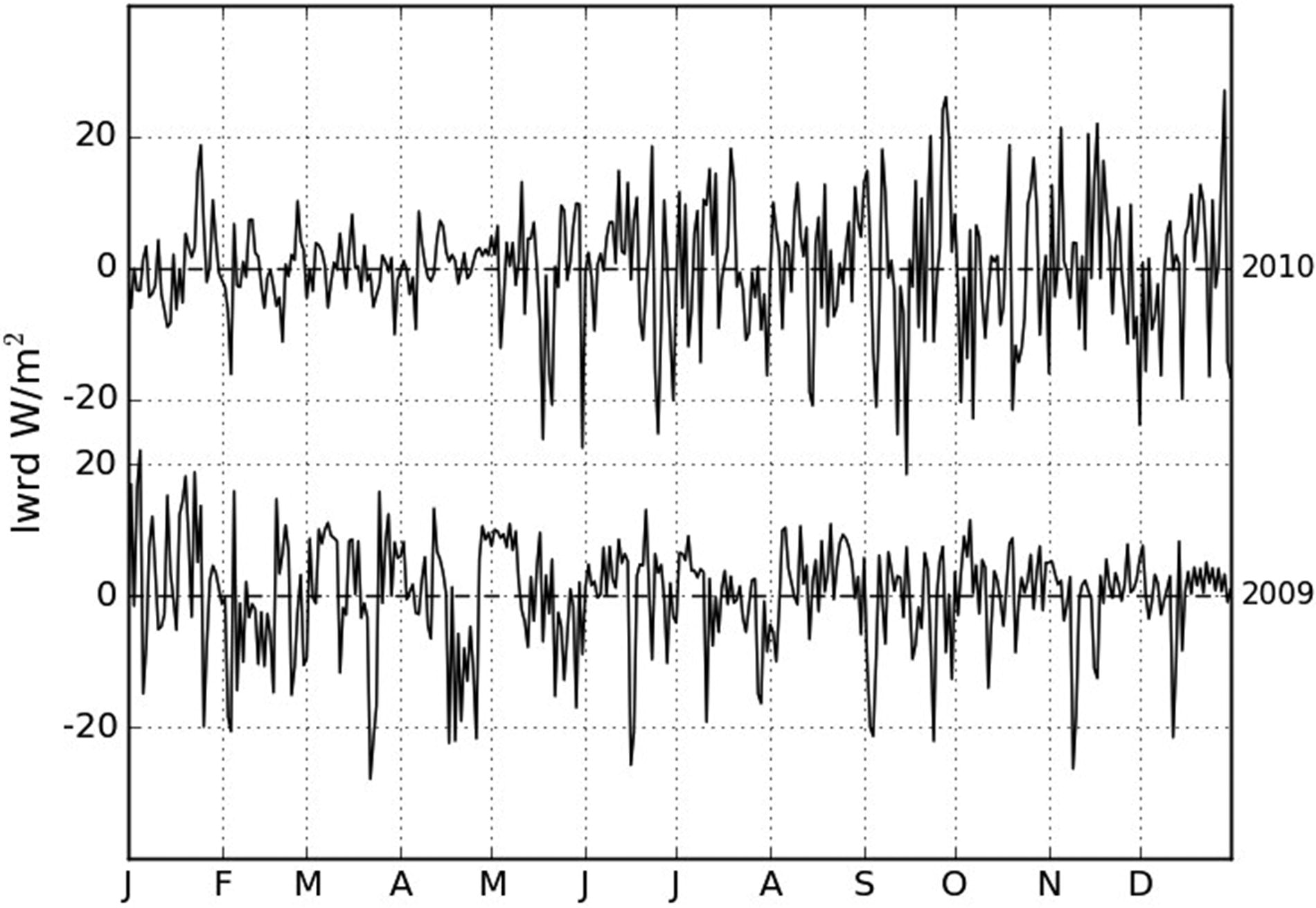
Fig. 7.
Training data for lwrd for the years 2009 and 2010 in the equatorial Pacific (0N, 180E).
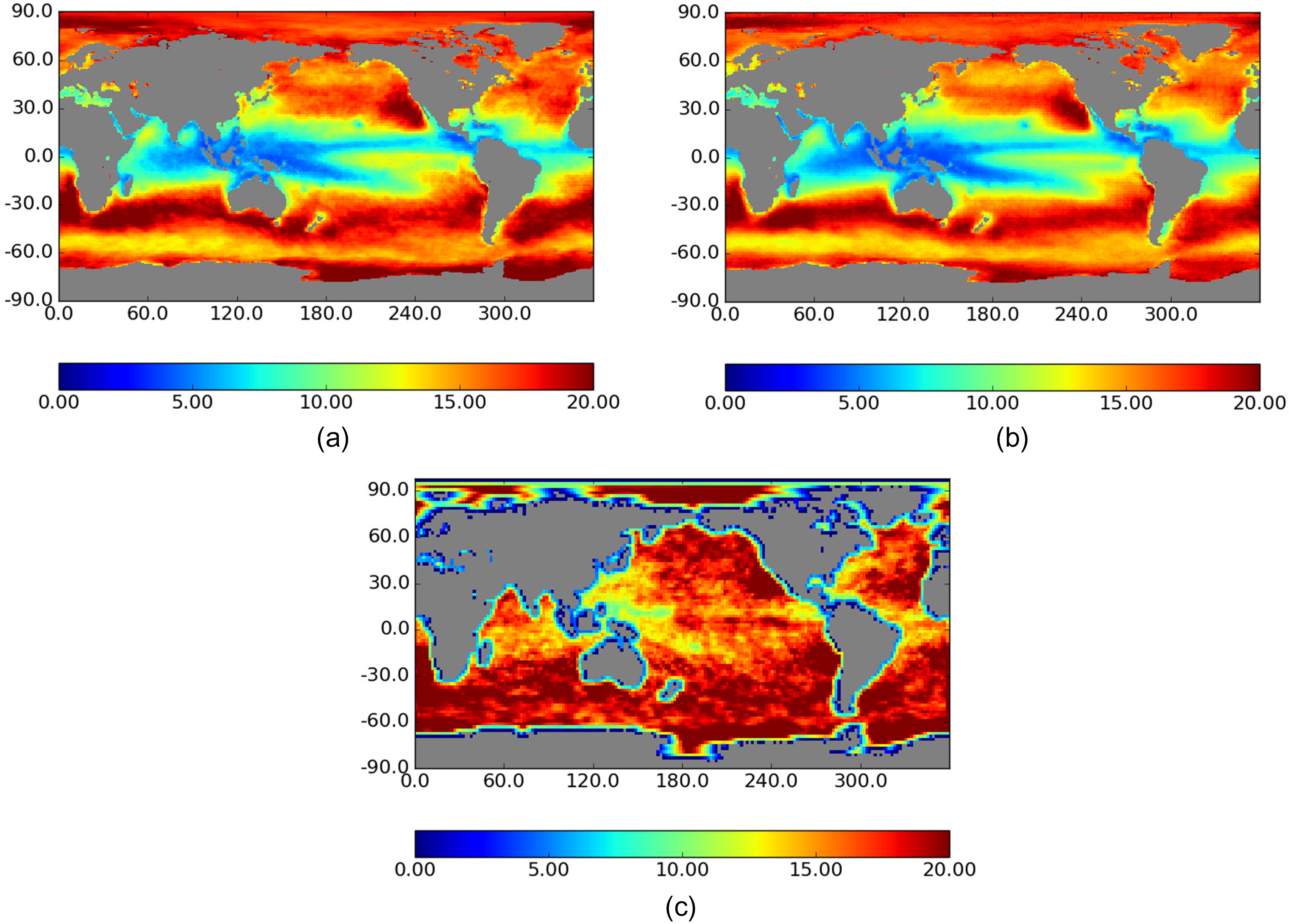
Fig. 8.
Standard deviation of lwrd for three years of original data (a), perturbations generated by the model (b), perturbations generated from the previous CMCC method (c).