
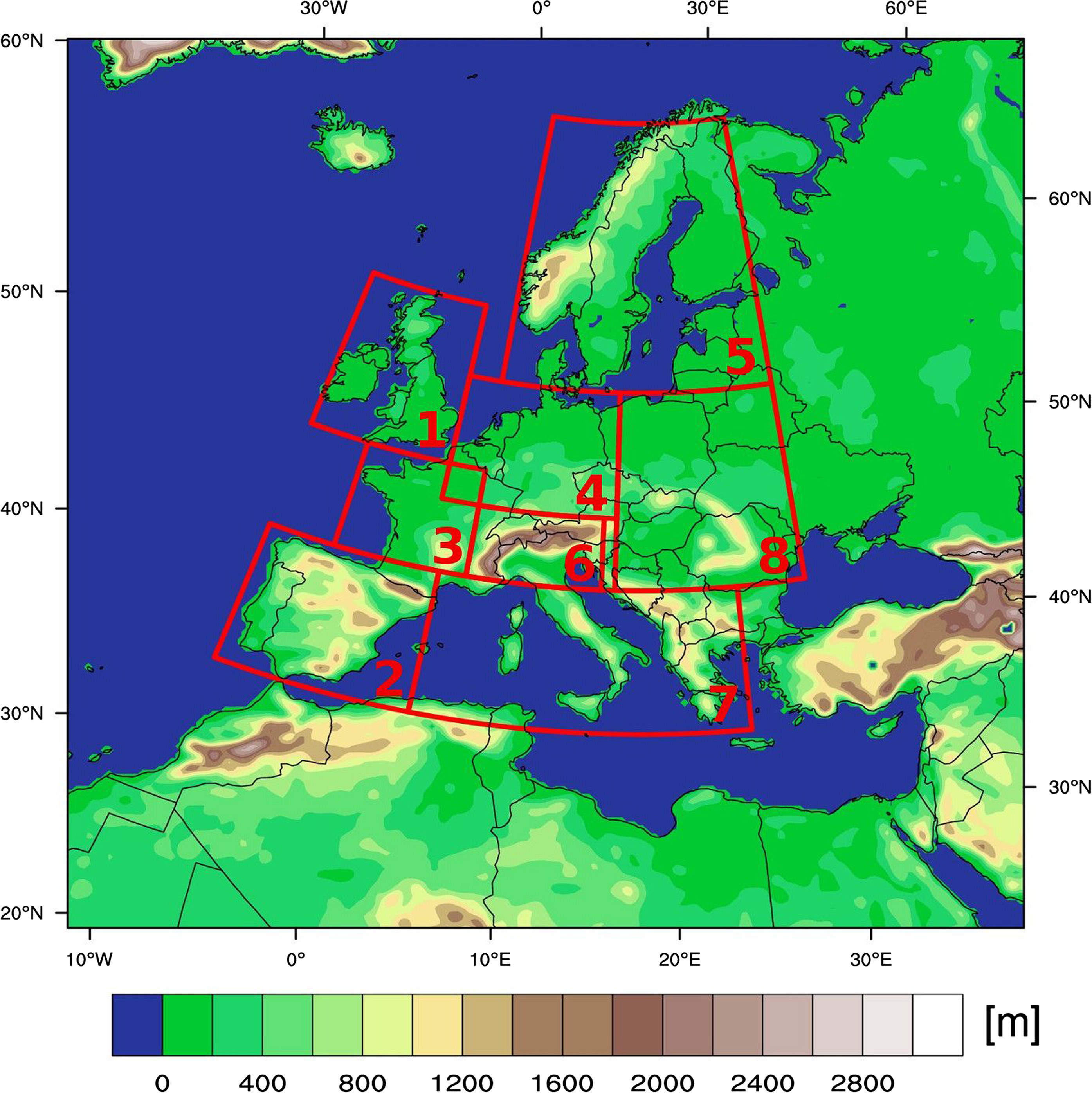
Fig. 1.
Model domain with topography for the EUR-44 grid and sub-regions – 1: British Isles (BI), 2: Iberian Peninsula (IP), 3: France (FR), 4: Mid-Europe (ME), 5: Scandinavia (SC), 6: Alps (AL), 7: Mediterranean (MD) and 8: Eastern Europe (EA).
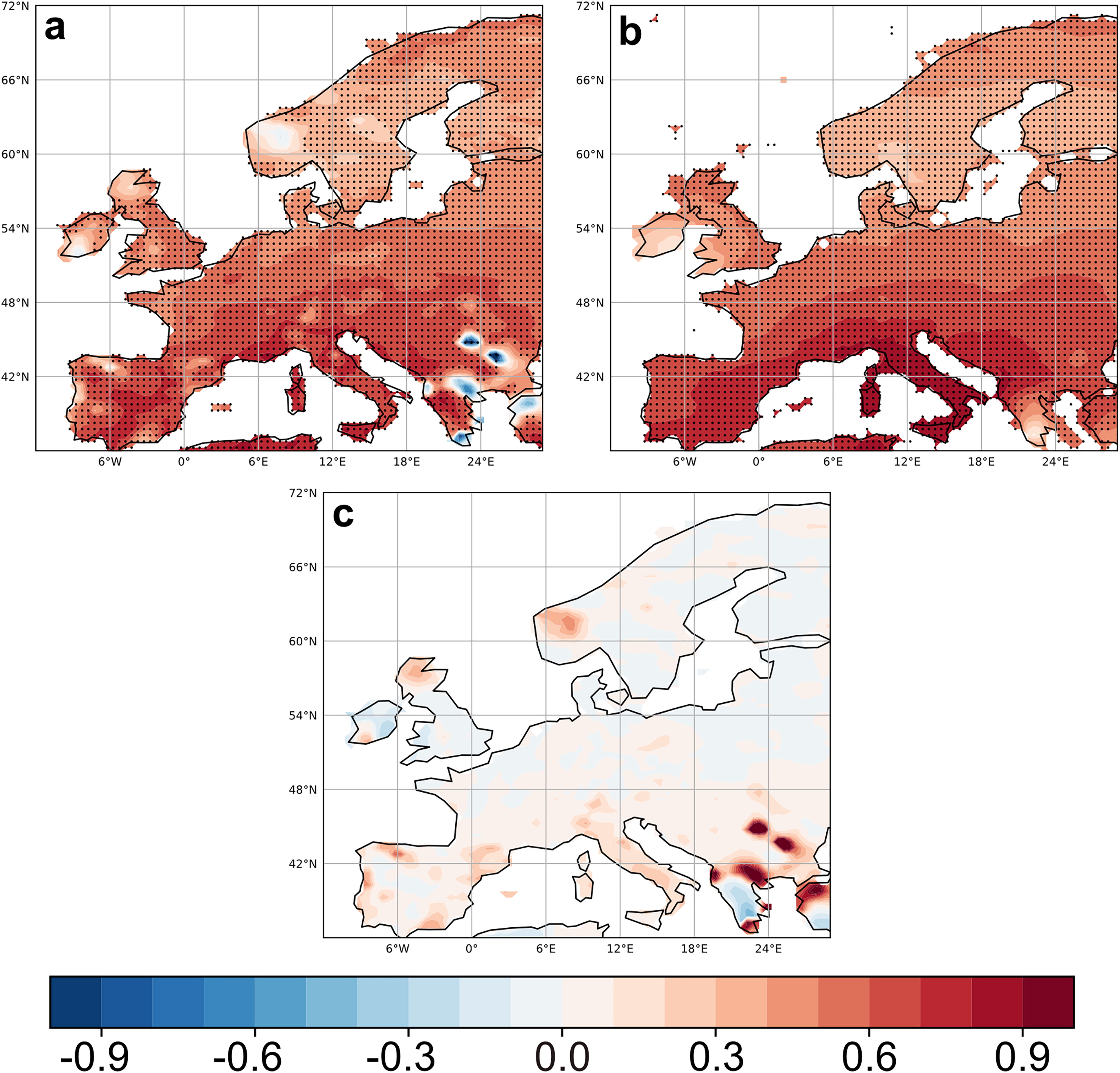
Fig. 2.
MSESS of CCLM hindcasts (average over lead-years 2–5) w.r.t. climatology derived from (a) E-OBS and (b) CRU TS4.01 for the period 1962–2015. The black dots indicate significant skill at the 95% level. (c) Difference MSESS CRU – MSESS E-OBS.
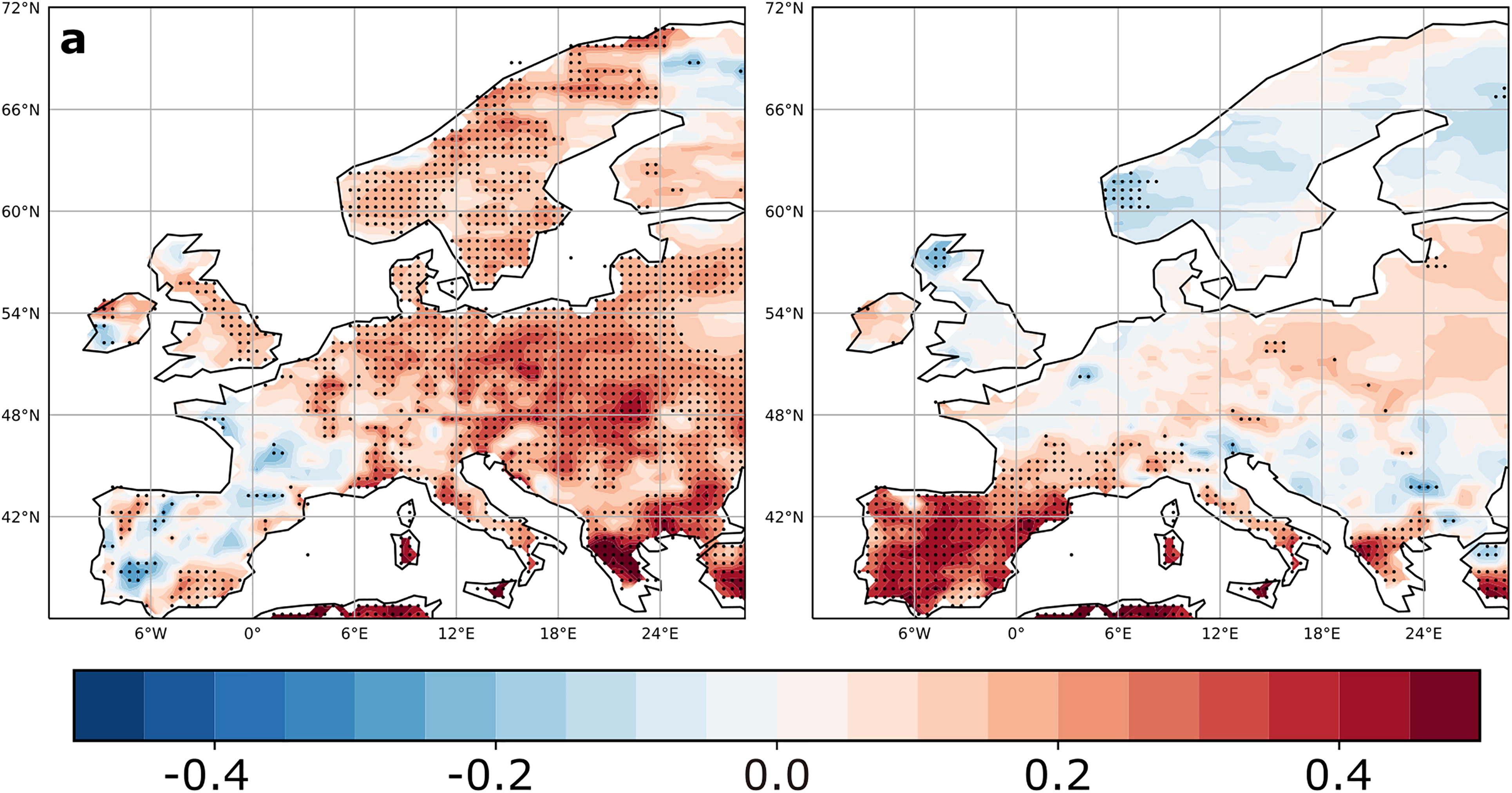
Fig. 3.
Skill and added value of downscaling: MSESS near-surface temperature (tas) compared to E-OBS; period 1967–2016, lead-time year 2–5. (a) MSESS CCLM b1 vs. MPI-ESM historical, (b) MSESS CCLM vs. MPI-ESM-LR b1.
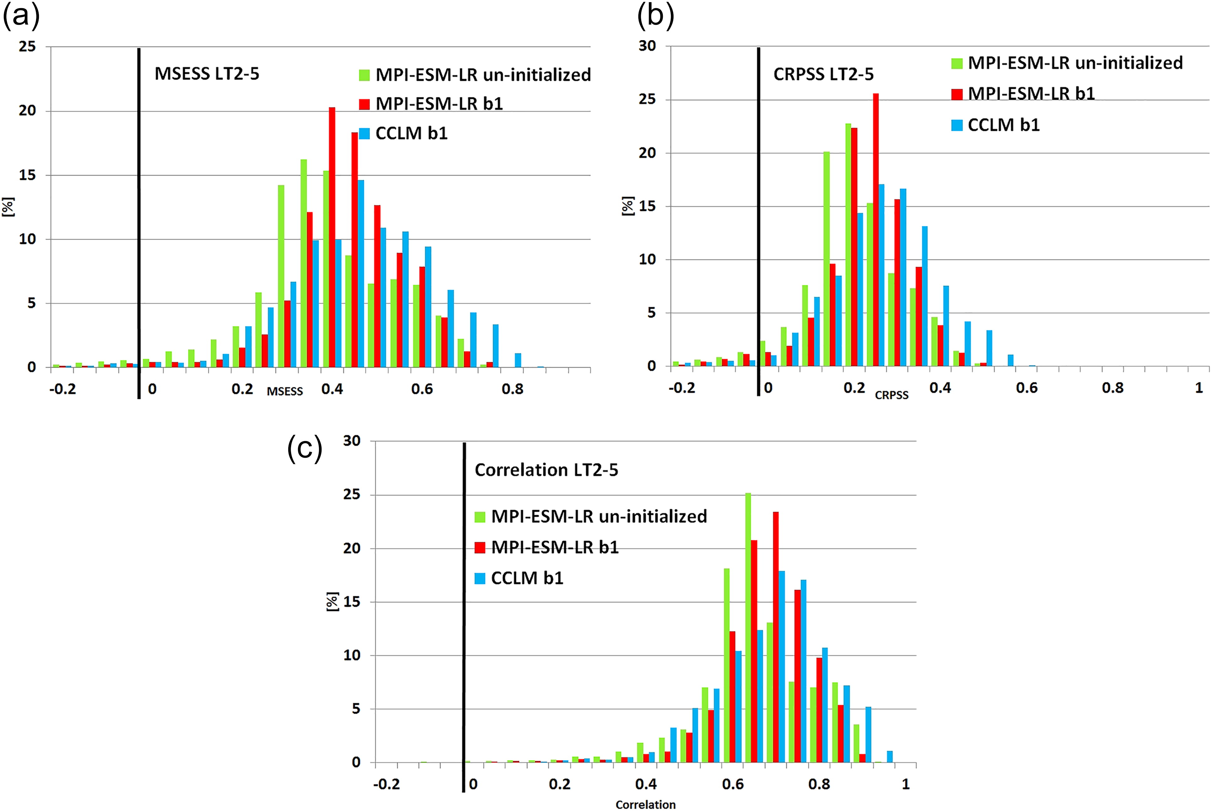
Fig. 4.
Skill distribution over Europe for lead-time years 2–5 for CCLM b1 (blue) and MPI-ESM-LR b1 (red) and MPI un-initialized (green). (a) MSESS, (b) CRPSS, (c) correlation (ACC).
Table 1.
Median and quartiles for the skill metrics (SM): MSESS, CRPSS and ACC compared to the E-OBS observations for regional CCLM b1 ensemble, the initialized MPI-ESM-LR b1 hindcast ensemble and the un-initialized MPI-ESM-LR historical simulations.
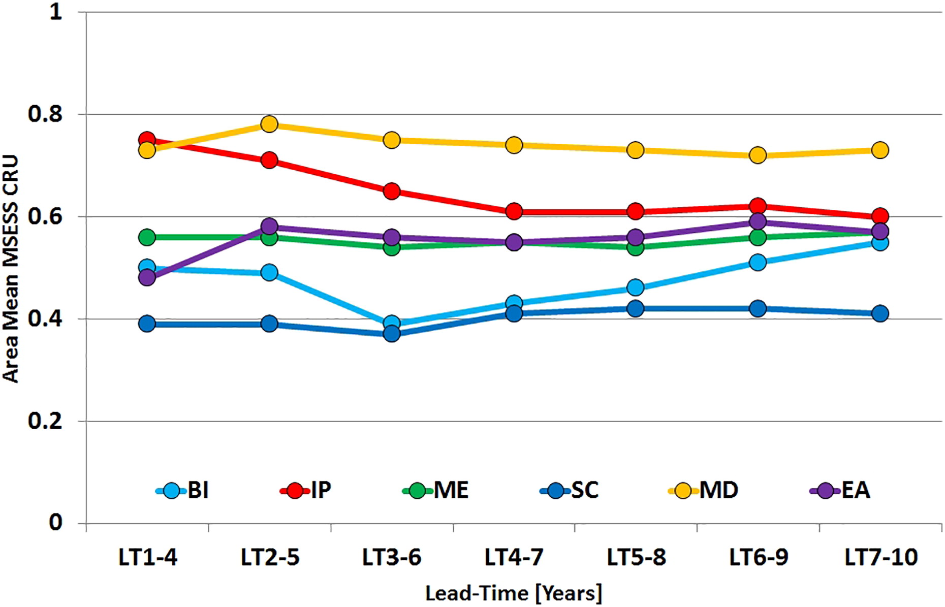
Fig. 5.
Lead-time dependence of MSESS for 4-year mean annual temperature in the CCLM hindcast ensemble as average over selected PRUDENCE regions (cf. Fig. 1) for the common verification period 1967–2015. The reference is the climatology of the CRU observations over the period 1967–2015.
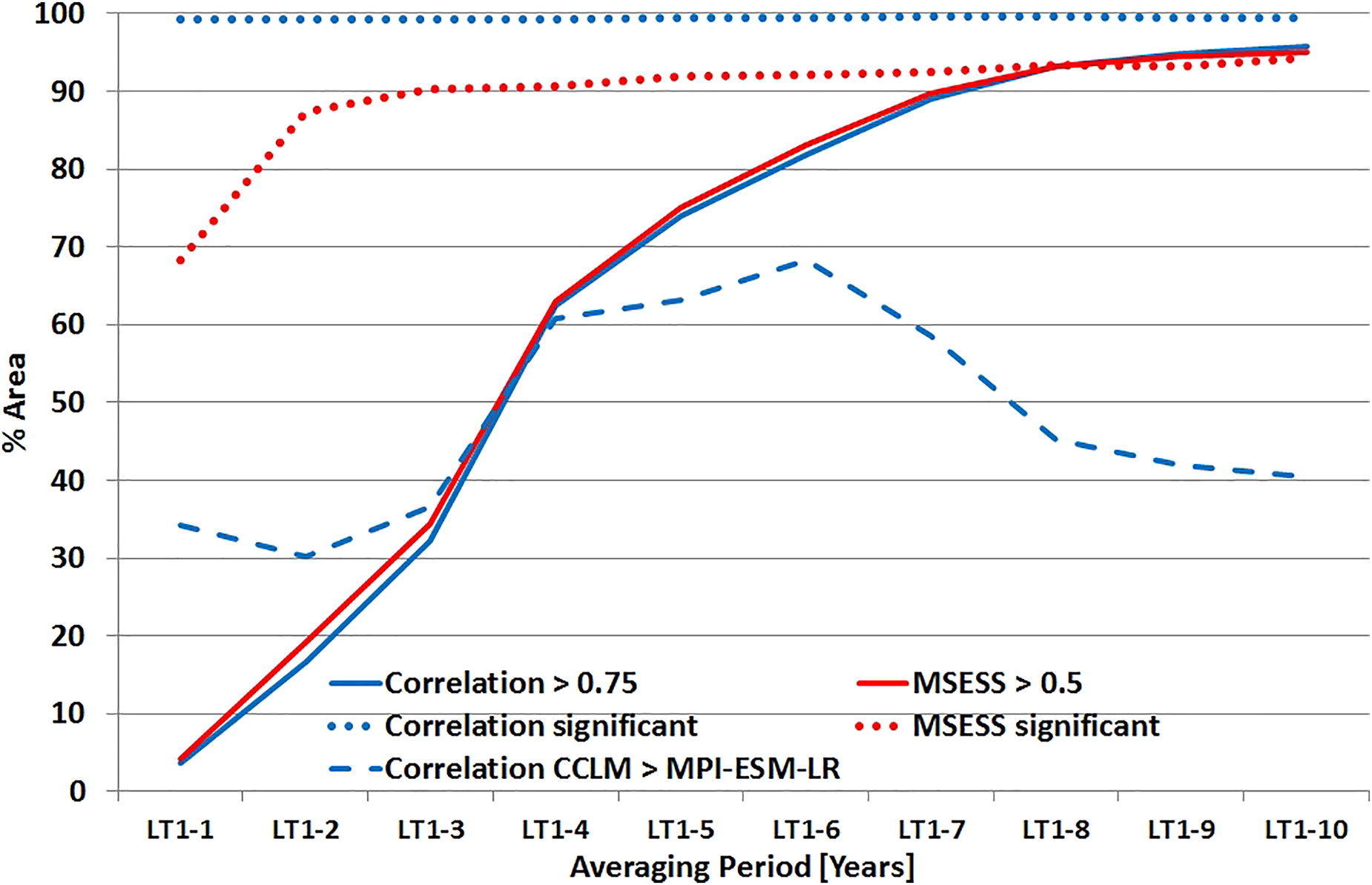
Fig. 6.
Area fraction of a considerable skill score in dependence to the averaging period (years) for near surface temperature from CCLM baseline1 ensemble 1961–2015. Anomaly correlation (blue); MSESS (red); area fraction with MSESS >0.5 and ACC >0.75 (solid lines), area fraction with skill significant at the 95% level (dotted), area fraction where skill of CCLM is higher than skill of MPI-ESM-LR (dashed).
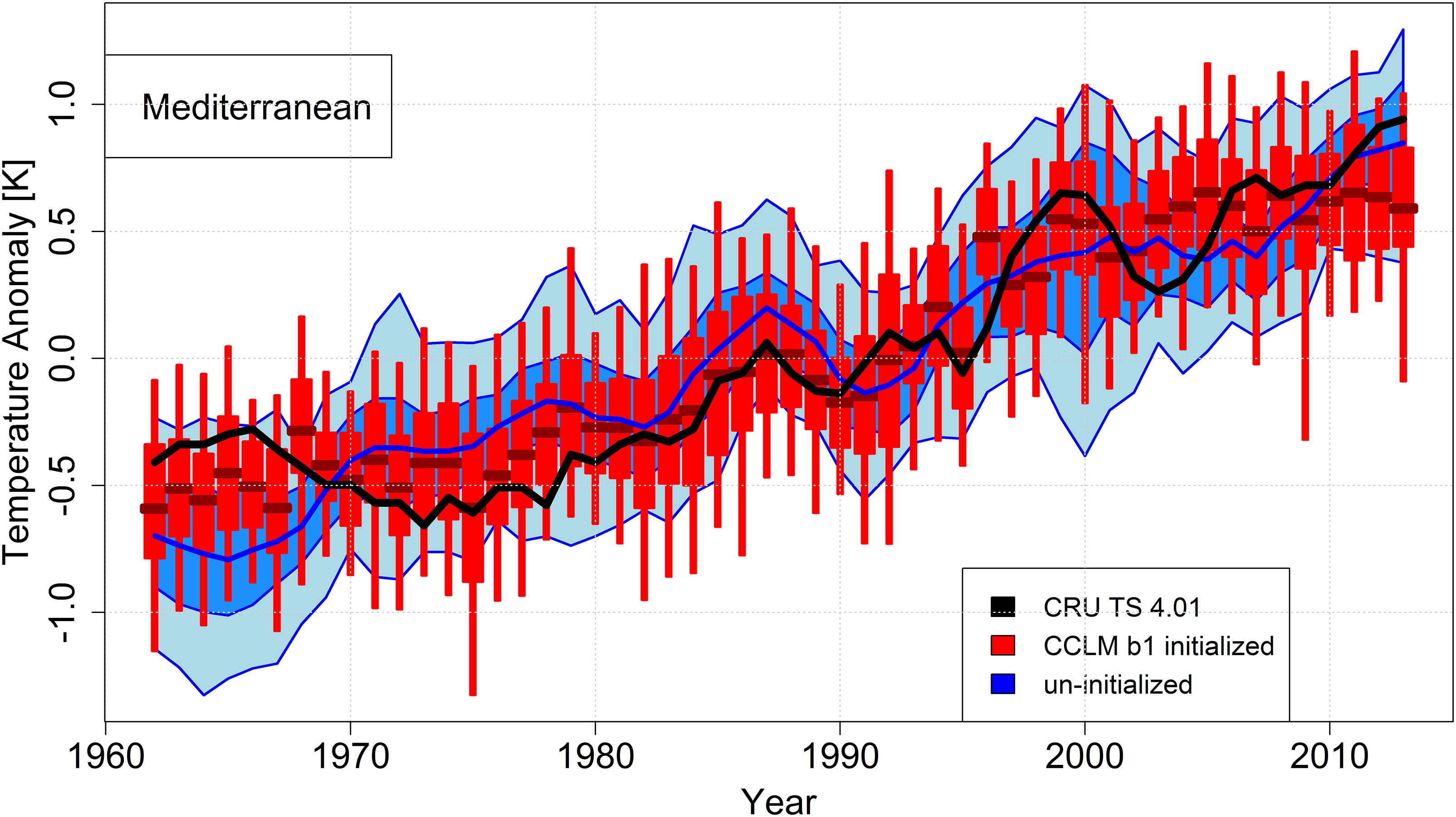
Fig. 7.
Temporal evolution of the 4-year mean annual temperatures in the Mediterranean region over the period 1962–2015 from CRU TS4.01 (black), the ensemble of historical simulations (blue), and the CCLM b1 hindcast ensemble (red) for lead-time years 2–5. The light blue area denotes the full range of the historical ensemble; the mid-blue area depicts the inter-quartile range and the dark blue line the ensemble mean. The red lines and boxes indicate the full and interquartile range of the hindcasts, the dark red lines the ensemble mean.
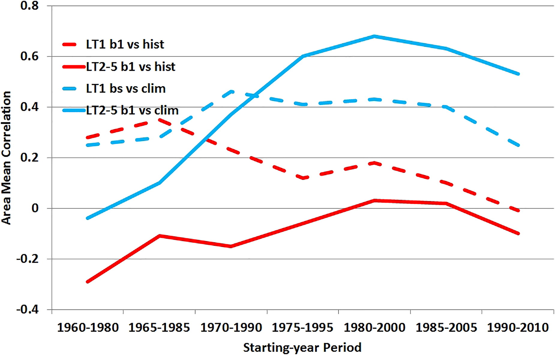
Fig. 8.
Ensemble mean correlation of the 4-year mean annual temperature of the regional baseline1 ensemble with the CRU TS4.01 observations for Europe. Anomaly correlation compared to climatology (blue lines) and the un-initialized simulations (red lines); differences between the correlation of the initialized and un-initialized ensembles – mean lead-years 2–5 (solid); lead-year 1 (dashed lines).
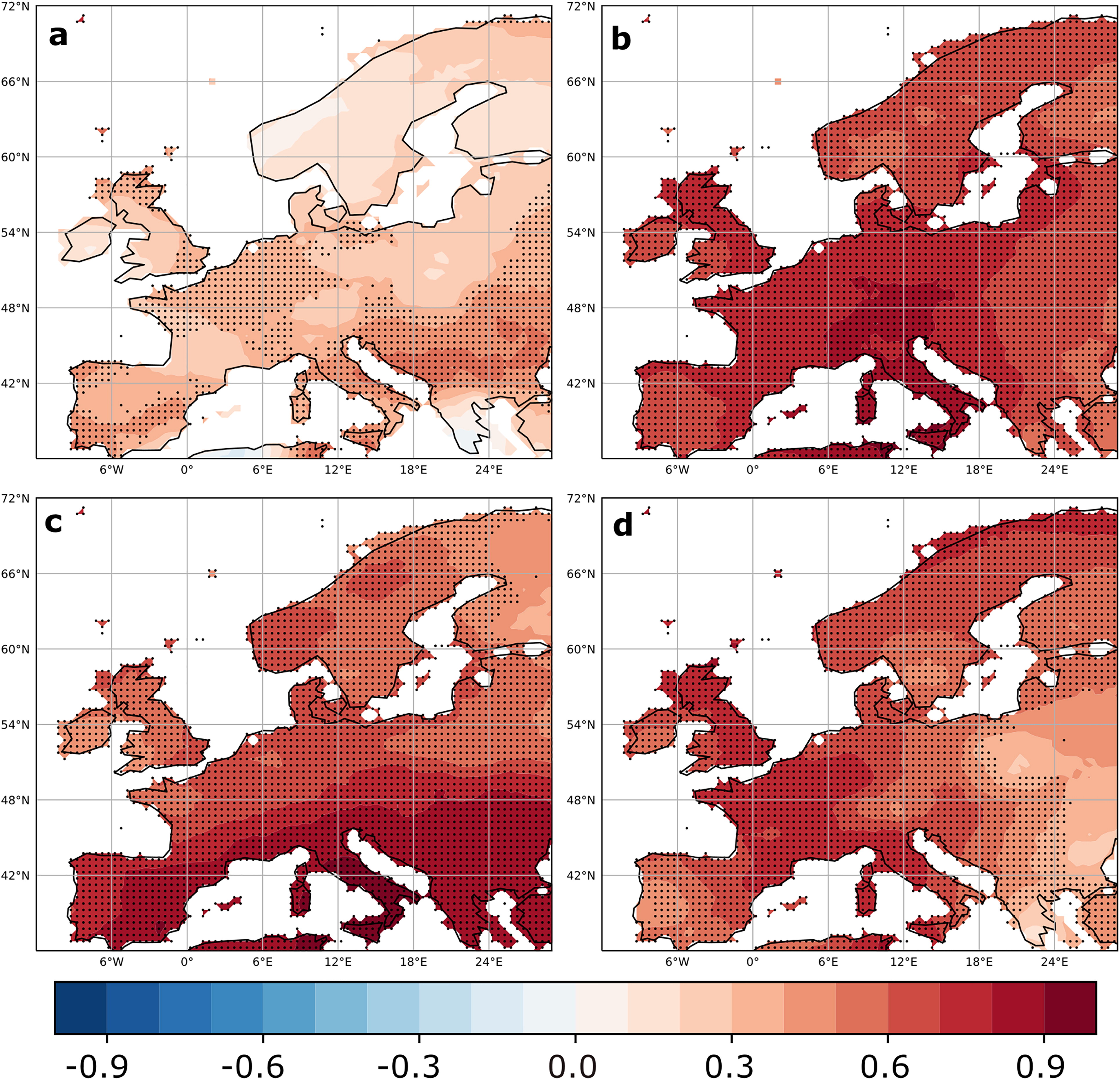
Fig. 9.
Correlation of seasonal 4-year mean temperature CCLM b1 lead-years 2–5 for the starting years 1960–2010 (analysis period 1962–2015). Observations CRU TS4.01, for (a) winter (DJF), (b) spring (MAM), (c) summer (JJA) and (d) autumn (SON).
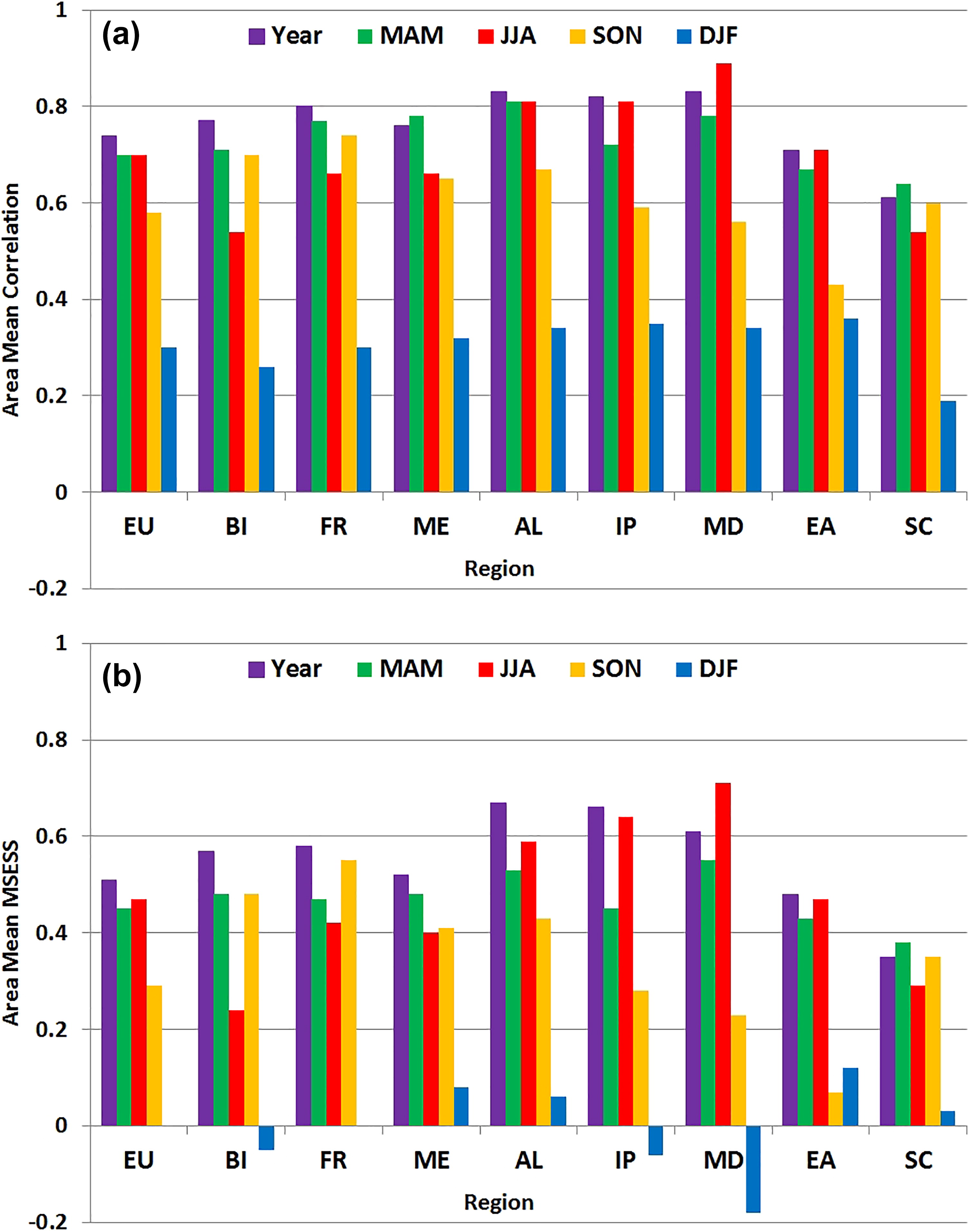
Fig. 10.
Area mean skill for 4-year mean temperature CCLM b1 lead-years 2–5 starting years 1960–2010. Correlation (a) and MSESS (b).
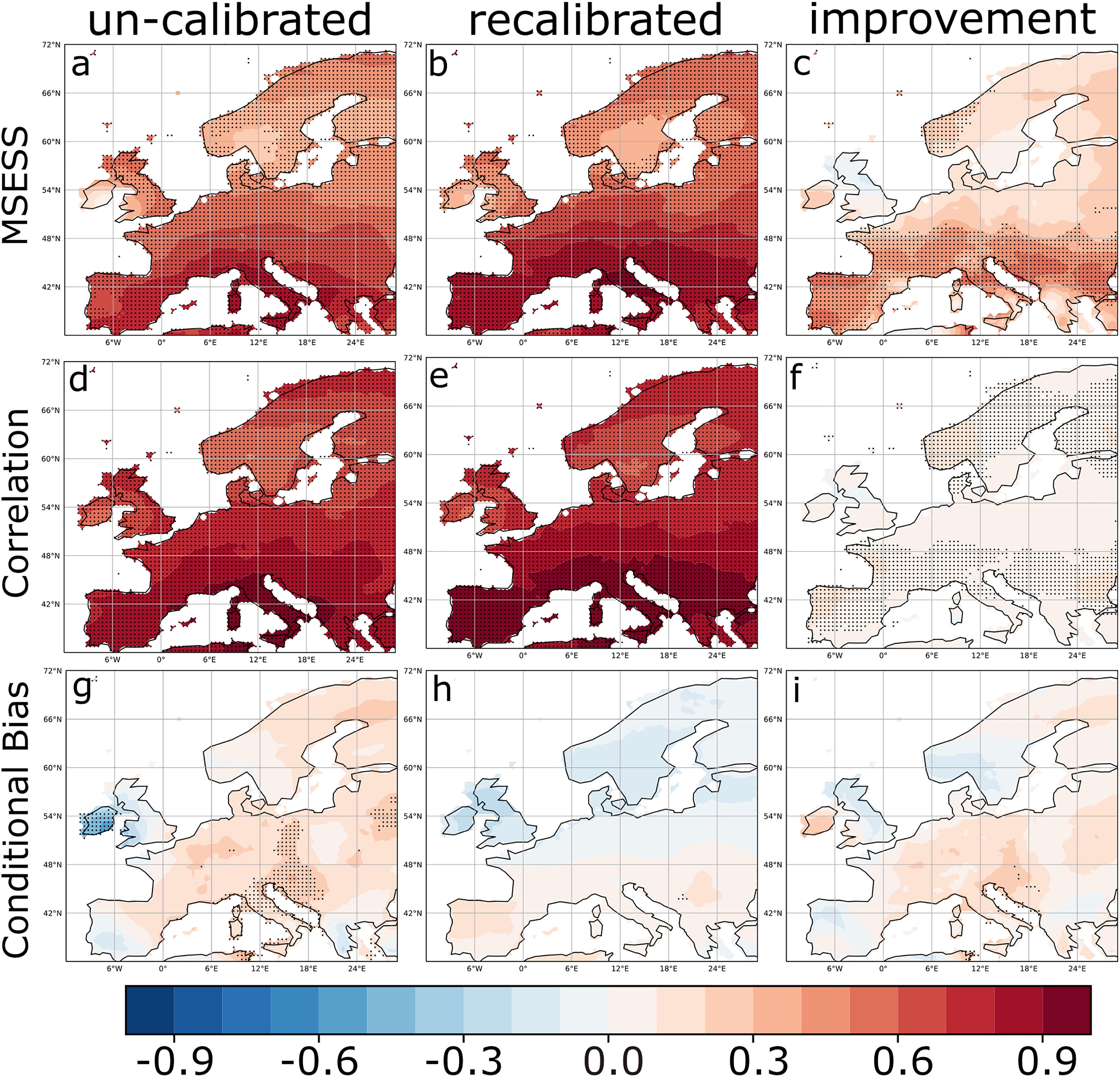
Fig. 11.
Comparison skill scores for temperature with and without recalibration. CCLM b1 ensemble, period 1967–2015, lead-time year 2–5. (a, d, g) Un-calibrated data. (b, e, h) Recalibrated. (c, f, i) Added value recalibration (as defined in Section 3). (a–c) MSESS. (d–f) ACC. (g–i) Conditional bias.
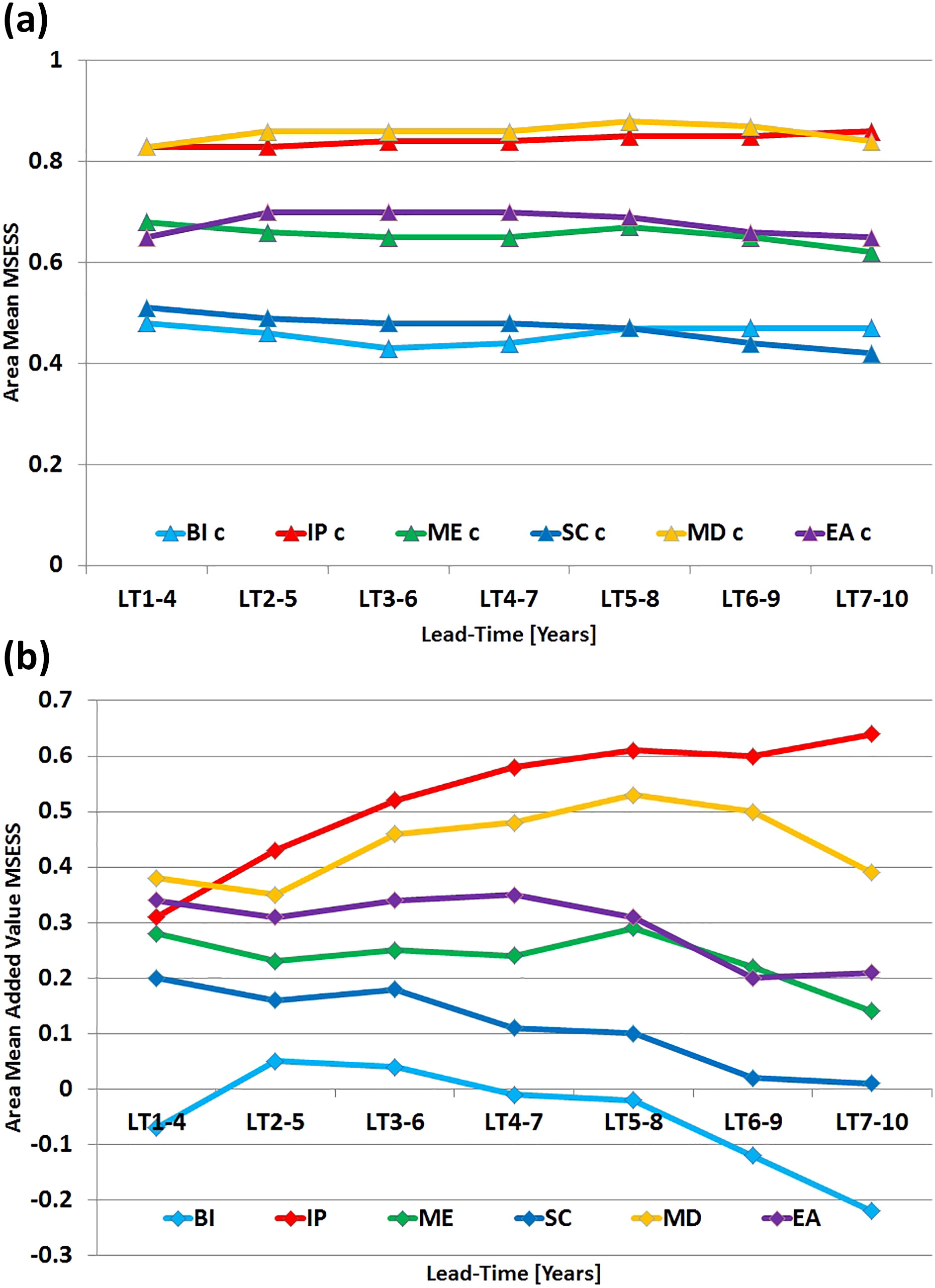
Fig. 12.
(a) Area mean MSESS CCLM b1 recalibrated 4-year mean temperature for different PRUDENCE regions and lead-times. Reference: climatology and CRU TS4.01 (cf. Fig. 6 for the un-calibrated hindcasts). (b) Added value MSESS for temperature of the calibrated with the uncalibrated CCLM ensemble as reference.
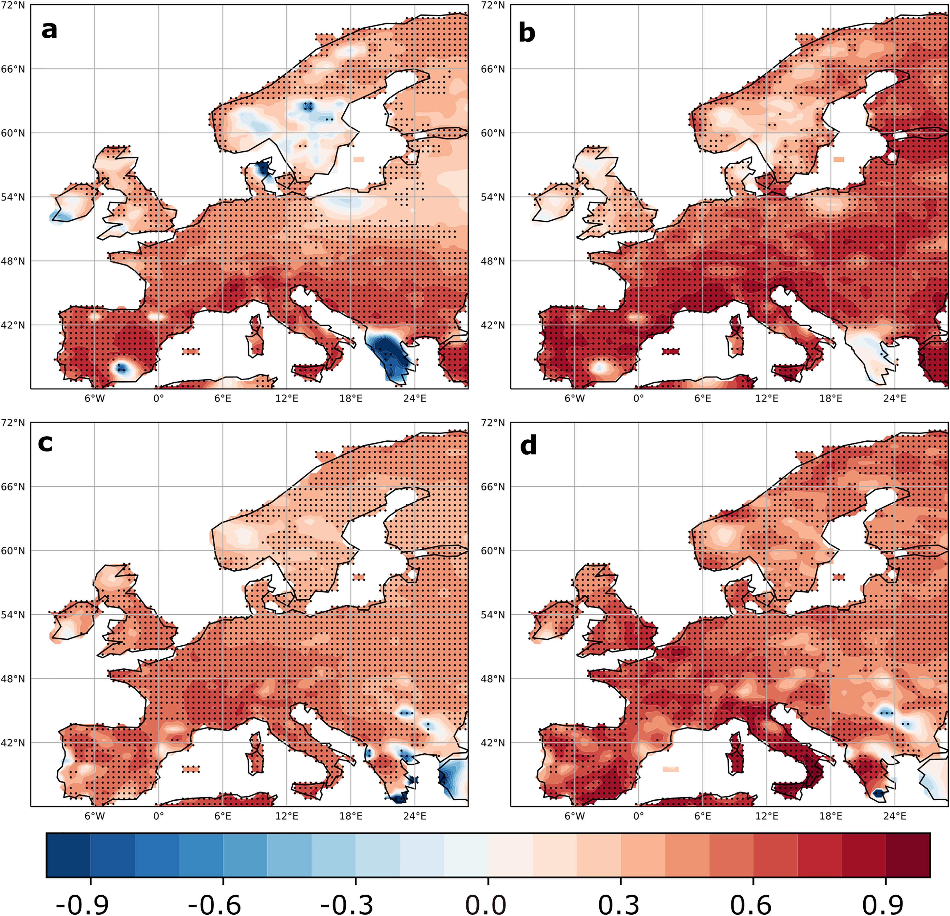
Fig. 13.
MSESS for CCLM b1 for the period 1967–2015 lead years 2–5. Daily maximum temperature JJA (a, b) and the heating degree days ( (c, d) un-calibrated (a, c) vs. calibrated data (b, d). Observational reference: E-OBS.