
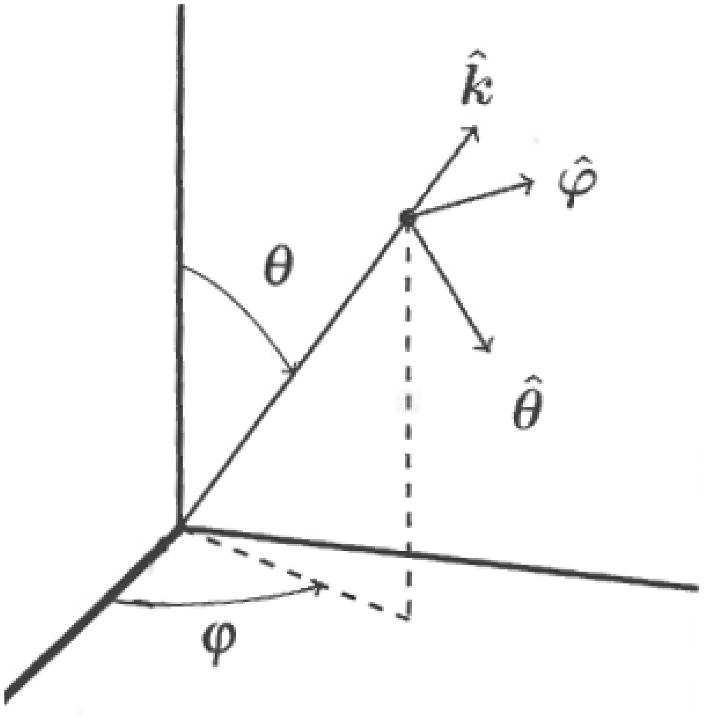
Fig. 1.
Schematic of the spherical polar co-ordinate system showing the unit vectors and that form a right-handed triad.
Table 1.
Parameter values used by LeBlond (1964) and WPA17.
Table 2.
Summary of calculated results for the frequencies of the planetary waves corresponding to azimuthal wavenumbers and –3. In the second and third columns are listed the frequencies given by numerical solutions of the full problem (4)–(5) and by the IT solution derived by evaluating all coefficients in (4) with In the remaining columns are listed the percentage errors in the IT solution (EIT) and the asymptotic result (6 b) taken to one, two and three terms (E1–E3).
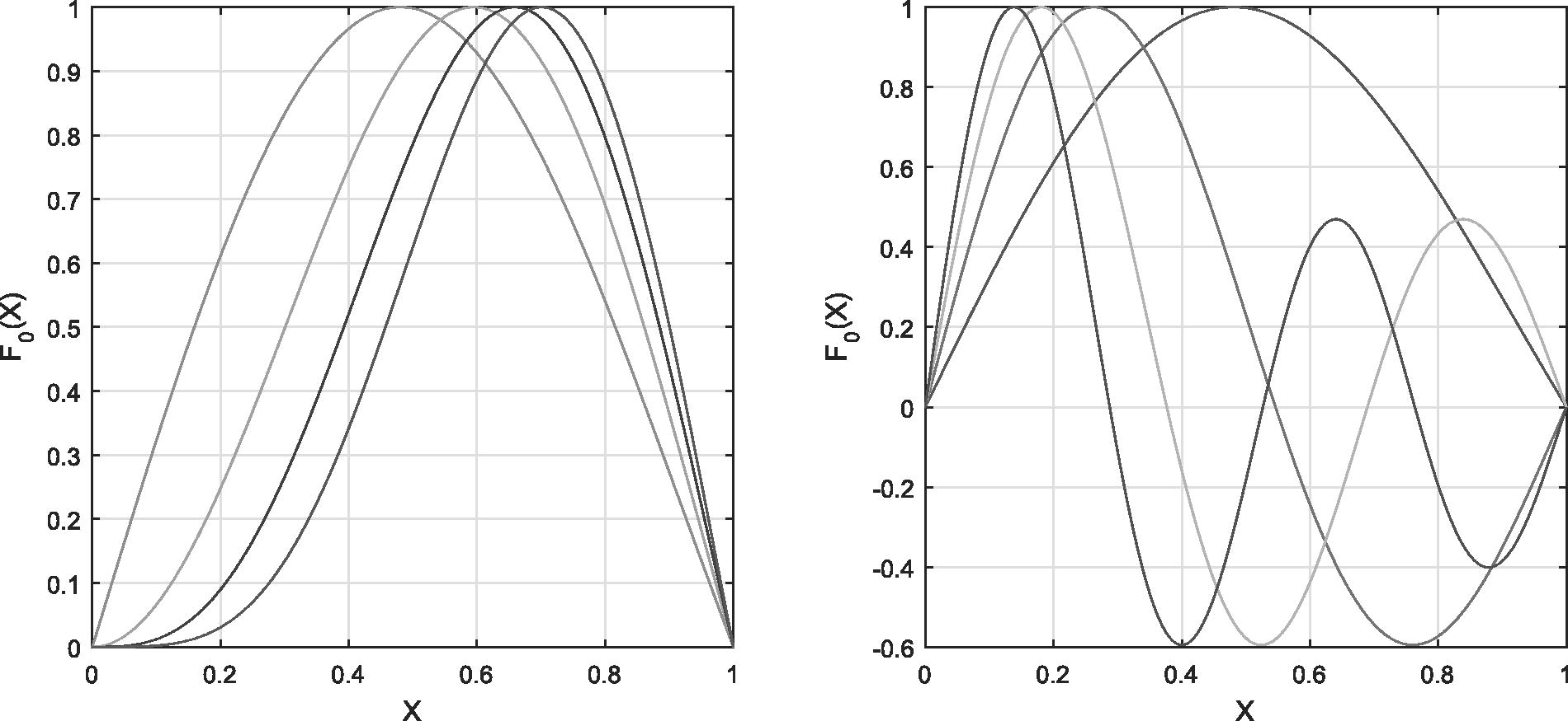
Fig. 2.
The form of the leading order eigenfunction given by solution (8) and normalised so as to have maximum value unity. The left panel shows the form of for n = 1 and M = 1 (leftmost curve), 2, 3 and 4 (rightmost curve). In the right panel is shown with M = 1 and with the nth mode having n – 1 interior zeros.
Table 3.
Summary of calculated results for gravity wave frequencies for azimuthal wavenumbers ±2 and ±3. The second and third columns give the numerically determined values using the full equation and the IT approximation. Remaining columns list the predicted frequencies using the two and three term series taken from (24) and their respective associated errors.
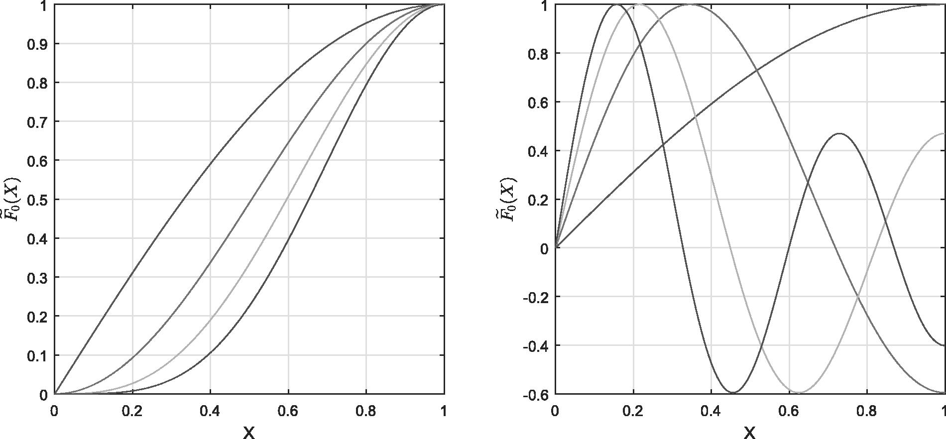
Fig. 3.
The form of the leading order eigenfunction given by solution (19) and normalised so as to have maximum value unity. The left panel shows the form of for n = 1 and (leftmost curve), 2, 3 and 4 (rightmost curve). In the right panel is shown with and with the nth mode having n – 1 interior zeros.