
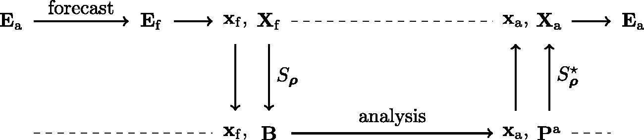
Fig. 1.
Sequence of steps of a deterministic EnKF with covariance localisation, where the updated perturbations are obtained using the new scheme. Note that and need not be fully computed.
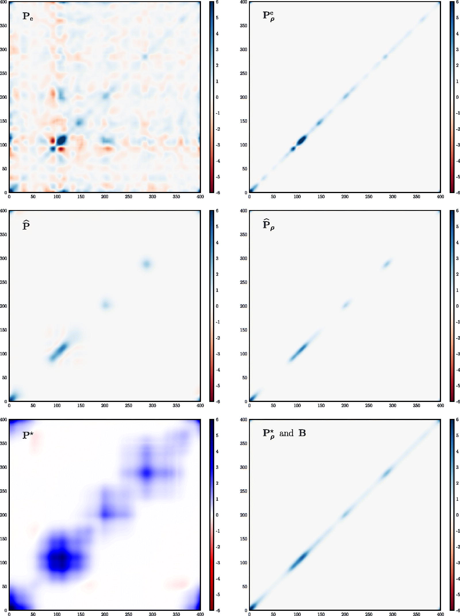
Fig. 2.
Density plots of the covariance matrices discussed in the text, except for and The raw sample covariance matrices are on the left, while the regularised (by localisation) sample covariance matrix are on the right. The true covariance matrix () cannot be visually discriminated from (bottom-right corner).
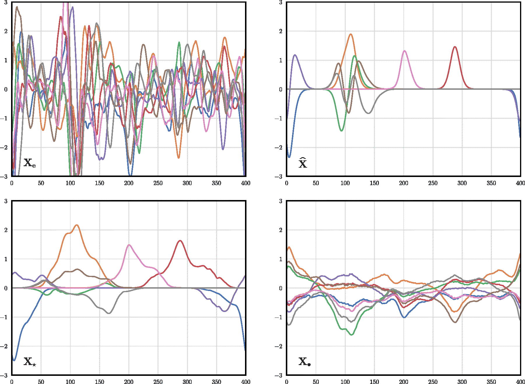
Fig. 3.
Plot of the perturbation sets: and with respect to the grid-point index.
Table 1.
Averaged Frobenius norm that measures the discrepancy between the target covariance matrix and several raw (first row) or regularised (second row) sample error covariance matrices.
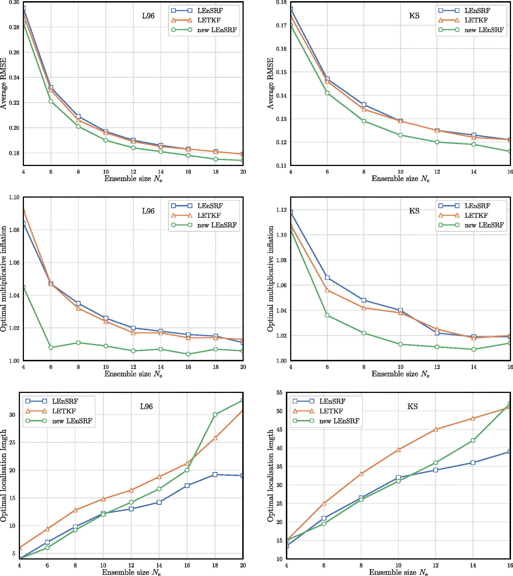
Fig. 4.
Comparison of the LETKF, the LEnSRF and the LEnSRF with the new update scheme, applied to the L96 model (left column) and to the KS model (right column). The RMSE, optimal localisation and optimal inflation are plotted as functions of the ensemble size
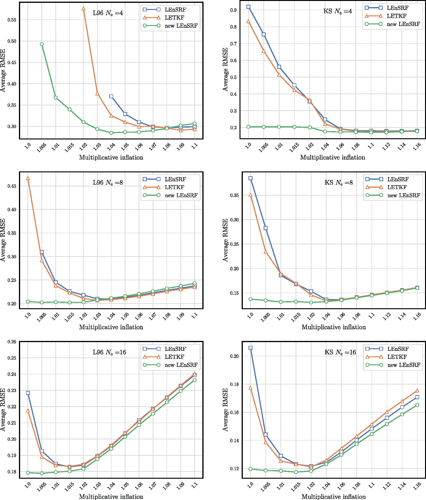
Fig. 5.
Time-averaged RMSE as a function of the multiplicative inflation, the localisation length being tuned so as to minimise the RMSE. The L96 results are displayed on the left panels while the KS results are shown on the right panels, for An absent marker means that at least one of the 10 sample runs has diverged from the truth.
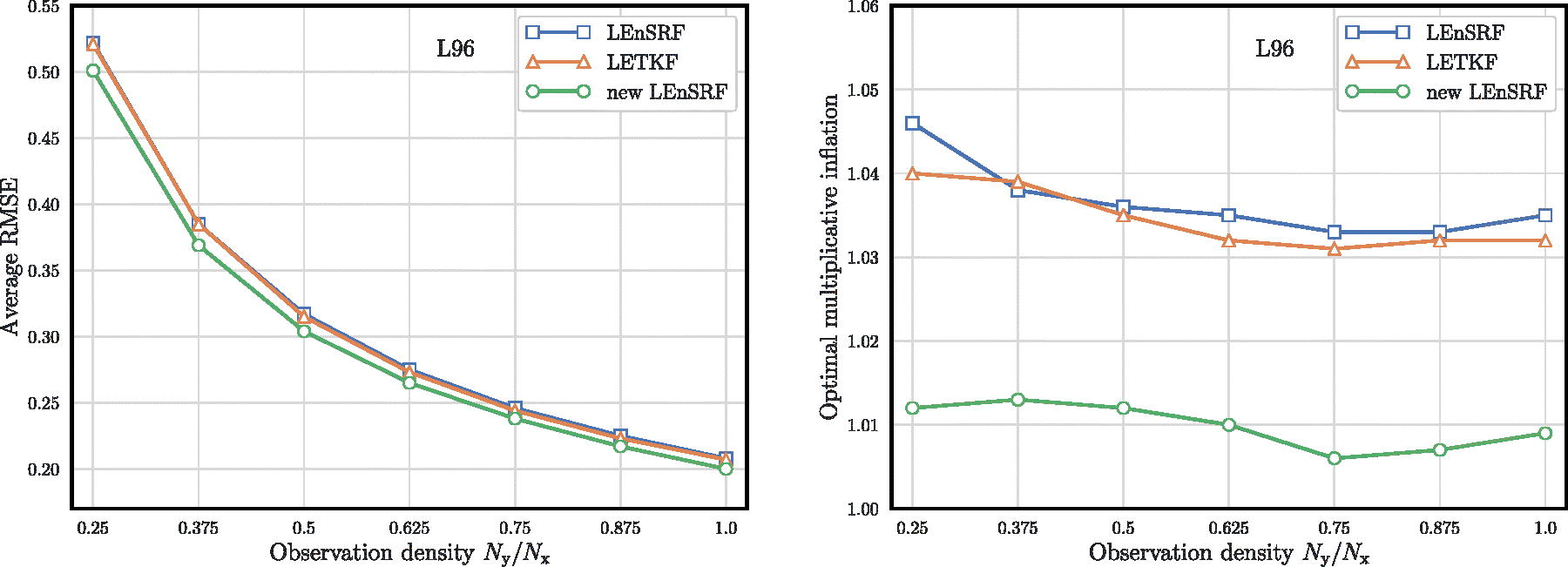
Fig. 6.
Comparison of the LETKF, the LEnSRF and the LEnSRF with the new update scheme, applied to the L96 model, for a fixed ensemble size and a fixed observation time step The RMSE (left panel) and the optimal inflation (right panel) are plotted as functions of the observation density
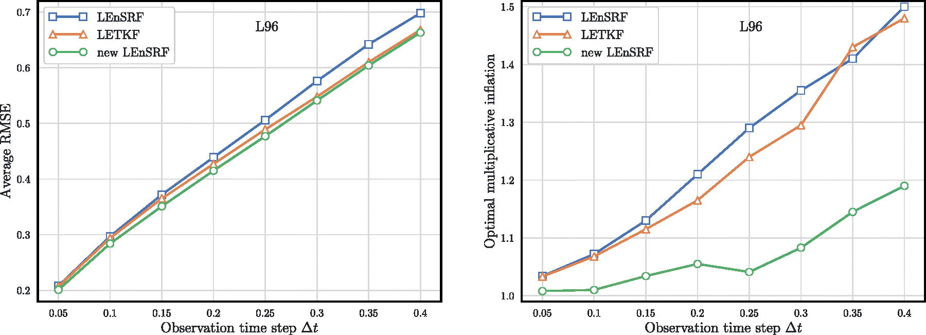
Fig. 7.
Comparison of the LETKF, the LEnSRF and the LEnSRF with the new update scheme, applied to the L96 model, for a fixed ensemble size and a fully observed model. The RMSE (left panel) and the optimal inflation (right panel) are plotted as functions of the observation time step
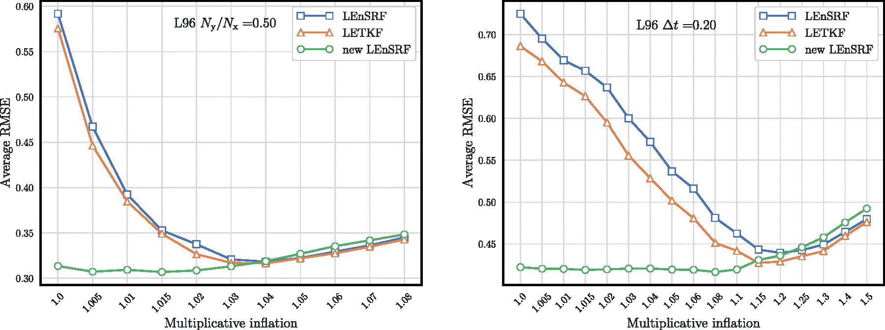
Fig. 8.
Time-averaged RMSE for the L96 model as a function of the multiplicative inflation, the localisation length being tuned so as to minimise the RMSE in the two configurations where the observations are sparser ( left panel) and where the observations are infrequent ( right panel). in both configurations.
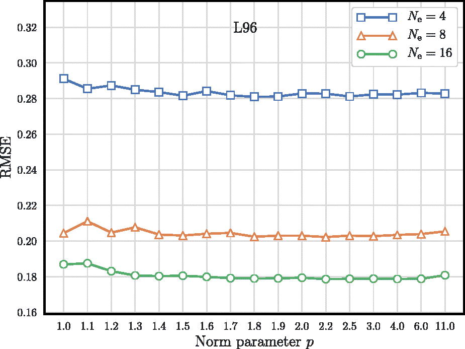
Fig. 9.
Average analysis RMSE as a function of the norm p parameter in the range and for and 16, applying the new LEnSRF scheme to the L96 model.